Forest stand delineation: turning canopy rasters into management polygons

Forests are managed in stands: patches of a few hectares where the trees are alike enough to be treated the same way, thinned in the same year or cut down together. Stand maps used to be drawn by hand on aerial photos and then fixed in the field. That’s slow, and two people rarely draw the same lines. Now that there’s LiDAR and drone imagery covering whole areas, a computer can suggest the borders. These notes go through the published ideas behind automatic stand delineation, plus a small synthetic example that shows the usual pipeline and where it struggles. It builds on the rasters from airborne LiDAR basics and the stand numbers in forest structure from above.

What makes a stand a stand

A stand is uniform in the things that matter for management: species mix, age or development stage, height, density, and often how good the site is. It also has to be big and compact enough to manage. Forest agencies set a minimum mapping unit, usually somewhere between a few tenths of a hectare and a couple of hectares, and they avoid long thin slivers. Some borders are physical (roads, streams, the edge of a clear-cut). Others are gradual, like density slowly changing across a slope.

That’s what makes the problem a bit unusual. It’s image segmentation, but:

• the “objects” are defined by statistics over many trees, not by the value of a single pixel;
• the result has to follow size and shape rules, not just similarity;
• the reference maps are subjective themselves, so a perfect score isn’t possible.

Step 1: describe each spot with features

One CHM pixel tells you almost nothing about the stand. It’s either a crown or a gap. The useful signal is in the statistics over a neighbourhood a few trees wide. Common features, computed over a moving window or per grid cell of 10–20 m, are:

• Height: mean, a high percentile like the 90th or 95th (close to dominant height), maximum.
• Density and cover: share of returns or CHM cells above 2 m, number of detected tree tops per area.
• Structure: standard deviation of heights (roughness), crown size, how returns are spread vertically.
• Spectral: mean band values or indices from imagery. These carry most of the species info (conifer versus broadleaf, for example).

Scale the features to similar ranges before comparing them, or the one with the biggest units ends up deciding everything. Then smooth them with an edge-preserving filter, like a median filter, so the noise inside stands goes down while the steps between stands stay sharp.

Step 2: segment

The published methods fall into a few groups.

• Region growing and multiresolution segmentation. Start from seed pixels or single pixels, and keep merging neighbouring regions as long as the merged region stays uniform. In Baatz and Schäpe’s multiresolution segmentation (the core of eCognition and of most object-based image analysis, OBIA), the cost of a merge mixes spectral variation with a shape term that rewards compact, smooth regions. One “scale parameter” caps how much variation a segment can hold. Lots of stand studies use it on CHM plus imagery, for example Mustonen et al. (2008) and Koch et al. (2009).
• Graph-based segmentation. Think of pixels as nodes in a graph, with edge weights equal to feature differences. Felzenszwalb and Huttenlocher (2004) merge two regions when the edge between them is weak compared with the variation inside each one. A scale parameter pushes towards bigger regions. It’s fast and copes with both sharp and gradual borders.
• Superpixels, then merging. First chop the image into many small compact pieces (SLIC is the usual pick), build a graph of which regions touch, and merge similar neighbours. This splits the job into “find good local borders” and “decide which pieces go together”.
• Clustering in feature space. k-means, mean shift or self-organising maps group cells with similar features no matter where they are, and connected components then give the polygons. You have to add spatial coherence afterwards, by smoothing or merging, or the result looks speckled.
• Learned segmentation. With enough labelled stands, a CNN, or a classifier followed by a graph model (Dechesne et al., 2017, for single-species stands), can learn which feature changes matter. Getting reference data is the bottleneck.
• Optimisation. Some forestry work treats delineation as an optimisation problem, using cellular automata or heuristics that balance within-stand uniformity against stand size, shape and even management goals.

Step 3: enforce the minimum mapping unit

Every method above leaves small leftover pieces: gaps, single big trees, transition zones. The usual fix is to merge each segment below the minimum area into its most similar neighbour, smallest first, until none are left:

import numpy as np
from scipy import ndimage as ndi

def absorb_small(labels, feats, min_cells):
    """Merge every segment smaller than min_cells into its most similar neighbour."""
    labels = labels.copy()
    while True:
        ids, counts = np.unique(labels, return_counts=True)
        if counts.min() >= min_cells:
            return labels
        s = ids[np.argmin(counts)]                              # smallest first
        ring = ndi.binary_dilation(labels == s) & (labels != s) # its neighbours
        f_s = feats[labels == s].mean(0)
        best = min(np.unique(labels[ring]),
                   key=lambda n: np.linalg.norm(feats[labels == n].mean(0) - f_s))
        labels[labels == s] = best

After that, turn the label raster into polygons, smooth or simplify the staircase edges, and snap them to hard borders like roads and property lines where you have them. The vector part is the same as in instance masks to polygons.

A synthetic example

I built a 200 m × 200 m CHM at 1 m resolution with five stands that differ in tree height, crown size and density, including a round young stand. The features were mean height, height standard deviation and canopy cover over a 21 m window, median-filtered. Then I ran graph-based segmentation with a 0.15 ha minimum unit.

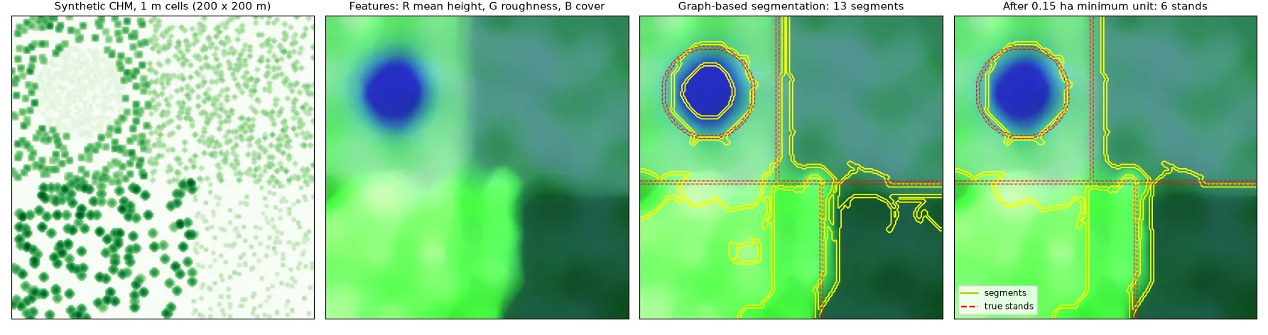
The result shows the typical behaviour. Strong contrasts, like young versus mature forest, come out almost exactly right. The part that surprised me was the moving window: it creates a transition band at every border, about one window wide (half a window on each side), where the features are a mix of both stands. The segmenter likes to cut that band out as its own thin segment, and then the minimum-area rule has to decide where it goes. Two stands with similar features stay hard to split no matter how you tune things, simply because the features don’t differ enough. Window size is the main trade-off: bigger windows give cleaner features inside stands, but blurrier, shifted borders.

How do you check a stand map?

Since the reference borders are subjective, you look at it from a few angles:

• Overlap per reference stand: for each reference polygon, find the segment that overlaps it most and report the shared area. Clinton et al. (2010) list the standard over- and under-segmentation measures built this way.
• Boundary distance: the share of predicted border that falls within some tolerance (say 10 m) of a reference border.
• Homogeneity: the within-stand variance of the things that matter (height, volume, species share), compared with the manual map. A map can disagree with the human interpreter and still be better for planning.
• Usability: number of stands, size distribution and how compact the shapes are, checked against the agency’s rules.

Key takeaways

• A stand is defined by statistics over many trees plus size and shape rules, so delineation means segmenting neighbourhood features, not raw pixels.
• Height percentiles, cover and roughness from LiDAR, plus spectral features for species, are the usual inputs. Scale them, and smooth with an edge-preserving filter.
• Region growing (multiresolution segmentation), graph-based segmentation, superpixels plus merging, and clustering all work. The clean-up to a minimum mapping unit matters as much as which method you pick.
• Window size trades noise inside stands against sharp borders, and transition bands are the usual source of small fake segments.
• Check results with overlap, boundary distance and within-stand homogeneity together, because the reference itself is subjective.

Resources

• B. Koch, C. Straub, M. Dees, Y. Wang, H. Weinacker, “Airborne laser data for stand delineation and information extraction”, International Journal of Remote Sensing, 30(4), 2009.
• J. Mustonen, P. Packalén, A. Kangas, “Automatic segmentation of forest stands using a canopy height model and aerial photography”, Scandinavian Journal of Forest Research, 23(6), 2008.
• C. Dechesne, C. Mallet, A. Le Bris, V. Gouet-Brunet, “Semantic segmentation of forest stands of pure species combining airborne lidar data and very high resolution multispectral imagery”, ISPRS Journal of Photogrammetry and Remote Sensing, 126, 2017.
• M. Baatz, A. Schäpe, “Multiresolution segmentation: an optimization approach for high quality multi-scale image segmentation”, Angewandte Geographische Informationsverarbeitung XII, 2000.
• P. Felzenszwalb, D. Huttenlocher, “Efficient graph-based image segmentation”, International Journal of Computer Vision, 59(2), 2004.
• R. Achanta et al., “SLIC superpixels compared to state-of-the-art superpixel methods”, IEEE TPAMI, 34(11), 2012.
• N. Clinton et al., “Accuracy assessment measures for object-based image segmentation goodness”, Photogrammetric Engineering & Remote Sensing, 76(3), 2010.
• D. Diaz, stand_mapping, an open-source collection of stand delineation tools and benchmarks.