Forest structure from above: from tree heights and crowns to DBH, basal area and Lorey's height
What the standard forest numbers (DBH, basal area, stems per hectare, DGV, Lorey's height, dominant height) mean, how to compute them right, and how published models guess DBH and biomass from the tree height and crown size you can see from above.
A forester describes a stand with a handful of numbers: how thick the trees are, how many there are per hectare, how much ground their stems cover, and how tall they are. Most of these are defined at breast height, 1.3 m above the ground. And that’s exactly the part of the tree a drone or an airborne laser scanner can’t see. From above, you get tree height and crown size. So here I collected the standard definitions, fixed a few formulas that are easy to get wrong, and looked at published models that try to bridge the gap between “what we can see” and “what foresters need”.
The basic tree measurement: DBH
DBH (diameter at breast height, written or ) is the stem’s diameter 1.3 m above the ground, measured in centimetres with a calliper or a diameter tape. Pretty much everything else in forest measurement is built on it: basal area, volume, biomass and growth.
The other per-tree values are simpler. Height is from the ground to the tip. Crown base height (CBH) is the height of the lowest live branch, so crown length is and crown ratio is , a number between 0 and 1. Crown width is how wide the crown spreads, usually the average of two measurements at right angles.
Stand numbers, done carefully
Basal area of one tree is the area of its stem cut across at 1.3 m. With in centimetres, the radius in metres is , so
The stand’s basal area is the sum over the trees in a plot, divided by the plot area in hectares:
It’s easy to forget the division by . Without it you get square metres per plot, not per hectare.
Stems per hectare is on a fixed-area plot. Angle-count (relascope) sampling works differently, and this took me a moment: every counted tree stands for stems per hectare, where BAF is the basal area factor of the gauge. So and . Thin trees count for many stems, thick trees for few.
Mean diameters. Three are in common use, and they’re not the same number:
- the arithmetic mean ;
- the quadratic mean diameter , the diameter of the tree with average basal area;
- the basal-area-weighted mean diameter, called DGV in Swedish forest data (grundytevägd medeldiameter):
Each tree’s diameter is weighted by its basal area, so big trees count more. You’ll sometimes see a shortcut written as . That’s only right if is the plot sum of , not the per-hectare value. The ratio is safer.
Heights. The plain mean height gets dragged down by small trees stuck under the canopy. Lorey’s height weights each tree by its basal area, just like DGV:
Swedish data call it HGV (grundytevägd medelhöjd). It follows stand volume better than . Dominant height is the mean height of the 100 thickest trees per hectare. On a plot of hectares that means the thickest trees, so 10 trees on a 0.1 ha plot. Dominant height barely changes when a stand is thinned, which is why it’s used for site index: the dominant height a stand reaches at a reference age. It’s often modelled with a Chapman–Richards curve , where is stand age, the height it levels off at, a rate and a shape parameter.
Reineke’s stand density index compares the stem count to that of a stand with a reference mean diameter of 25 cm:
The exponent is positive. A version with floats around in some notes, but it makes a stand of big trees look less dense, which is the opposite of the whole point.
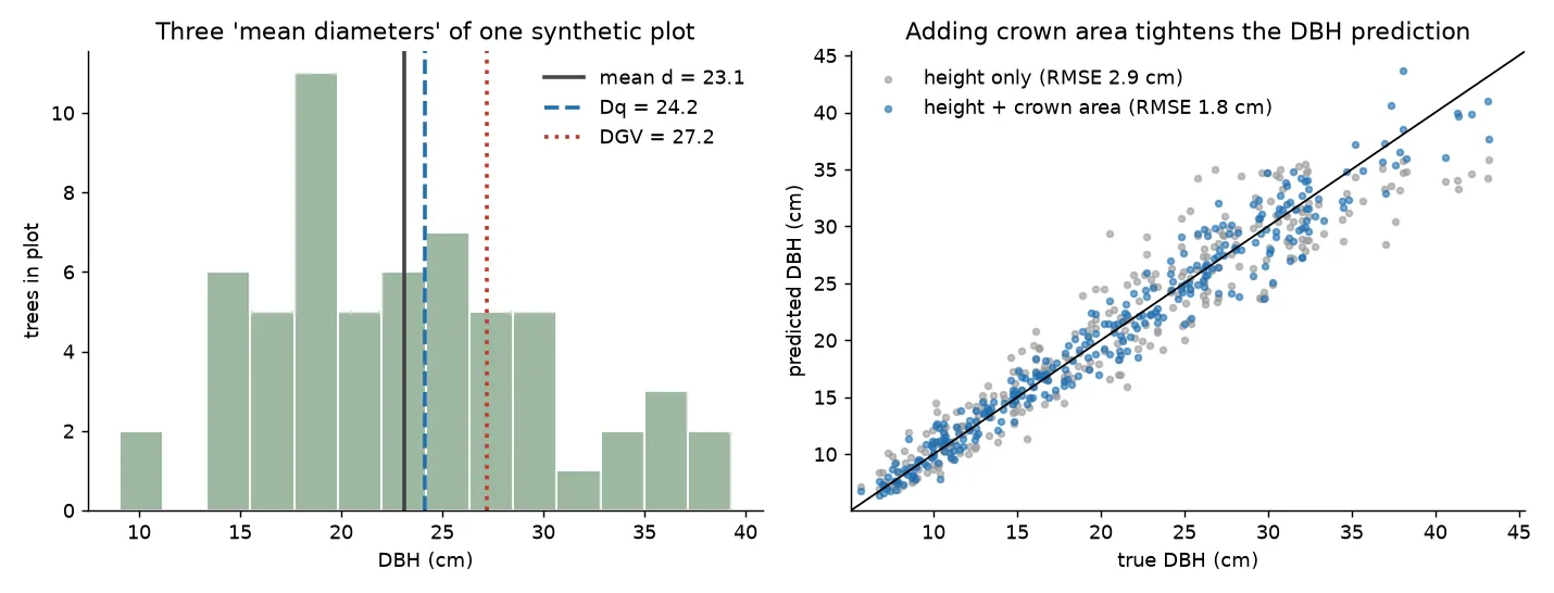
Here’s all of it on a synthetic plot:
import numpy as np

rng = np.random.default_rng(0)
A = 0.1                                       # plot area, ha
d = rng.gamma(shape=9, scale=2.6, size=60)    # DBH, cm
h = 1.3 + (d / (1.6 + 0.20 * d)) ** 2         # Näslund-type height curve, m

g   = np.pi * (d / 200) ** 2                  # basal area per tree, m²
G   = g.sum() / A                             # m²/ha
N   = len(d) / A                              # stems/ha
Dq  = np.sqrt((d ** 2).mean())
DGV = (g * d).sum() / g.sum()                 # = Σd³ / Σd²
H_L = (g * h).sum() / g.sum()                 # Lorey's height
H_dom = h[np.argsort(d)[-round(100 * A):]].mean()
SDI = N * (Dq / 25) ** 1.605
# N=600, G=27.5, mean d=23.1, Dq=24.2, DGV=27.2, mean h=14.7, H_L=15.9, H_dom=17.7
It’s always , and the gap gets bigger the more the diameters vary. The height model above is Näslund’s function , the classic height–diameter curve in Nordic forestry.
Bridging the gap: guessing DBH from height and crown
From a canopy height model and a crown segmentation you get, per tree, the height and the crown area (or radius ). Allometry is the idea that parts of a tree grow in proportion to each other, roughly following power laws. So a natural model is
which turns into a straight-line model once you take logs. Four published studies show the same lesson from different angles.
Chen et al. (2007), blue oak woodland in California, small-footprint LiDAR. They compared lots of models for single-tree basal area and stem volume. A linear DBH model from maximum height and crown area, (DBH in cm, the highest return in m, the crown area in m²), followed by , was among the best when crowns were segmented correctly. Their own new idea was the canopy geometric volume , the volume under the crown surface. They modelled basal area and stem volume as simple power functions of , and these held up best when the segmentation made mistakes.
Cao & Dean (2013) start from the uniform stress theory. The idea is that a stem tapers so that wind pushing on the crown causes about the same bending stress all along the stem. So the diameter at some height depends on the leaf area above it times the lever arm to the centre of that leaf area. With (height of the crown centre) and the lever arm m, they fit , where the leaf area is itself estimated from height and crown length. Both inputs come from LiDAR. Models with crown length clearly beat height-only power models, and adding stems per hectare helped all of them.
Gonzalez-Benecke et al. (2022), plantations of Pinus radiata, Eucalyptus globulus and E. nitens, built three levels of models for DBH (cm), stem volume and above-stump biomass: height only; height plus crown area; and height, crown area and stand variables like age and stems per hectare. Height-only models worked, but their errors grew with tree size. Adding crown area gave the biggest single improvement and got rid of that size bias.
Liu et al. (2024) skip DBH and predict above-ground biomass directly from height and crown radius measured from UAV data. The reference biomass came from standard equations. They tried nine forms. Models that used both and beat models with just one of them, and the quadratic was the most consistent across forest types (in mixed coniferous stands, ).
On synthetic trees where crown size carries real information, the effect is easy to see:
rng = np.random.default_rng(1)
H  = rng.uniform(8, 30, 300)                                   # tree height, m
CA = np.exp(rng.normal(np.log(0.12 * H**1.5), 0.35))           # crown area, m²
DBH = 1.2 * (H - 1.3)**0.75 * CA**0.30 * np.exp(rng.normal(0, 0.08, 300))  # cm

def fit_power(y, *xs):
    """Fit y = b0 * x1^b1 * x2^b2 ... by least squares on logs."""
    X = np.column_stack([np.ones_like(y)] + [np.log(x) for x in xs])
    b, *_ = np.linalg.lstsq(X, np.log(y), rcond=None)
    return b, np.exp(X @ b)

b1, pred1 = fit_power(DBH, H - 1.3)          # height only     -> RMSE 2.9 cm
b2, pred2 = fit_power(DBH, H - 1.3, CA)      # + crown area    -> RMSE 1.8 cm
Two things to watch out for. First, turning a log-scale fit back with exp gives you the median, not the mean, so it comes out a bit low. A correction factor like fixes most of that. Second, every coefficient is specific to a species and region. A model fitted to plantation eucalyptus tells you nothing about Swedish spruce until you refit it on local field plots.
From trees to stand values
The literature has two broad routes. In the individual-tree approach (for example Hyyppä et al., 2001), each detected tree gets a predicted DBH from models like the ones above. The stand numbers then come from summing , or over the trees in an area and dividing by that area. Its weak spots are trees hidden under the canopy, which never get detected, and crowns that get merged or split, which mess up both the tree count and the crown areas (see polygon validity and shape metrics for checking crown shapes). In the area-based approach (Næsset, 2002), stand values like , or volume are regressed straight on height statistics of the point cloud over field plots, with no tree detection at all. Hidden trees don’t hurt it much, but you don’t get a list of trees. When volume per tree is needed, it’s usually a species function .
Key takeaways
- Basal area per tree is m² with in cm. Divide the plot sum by plot area to get m²/ha.
- , and DGV are three different means. DGV and Lorey’s height both weight trees by basal area ( and ).
- Dominant height uses the 100 thickest trees per hectare. Reineke’s SDI uses a positive exponent of 1.605.
- Height alone predicts DBH and biomass with errors that grow for big trees. Adding crown size (area, radius or length) fixes a lot of that.
- Allometric coefficients are local: refit them with field data before trusting them.
Resources
- Chen, Q., Gong, P., Baldocchi, D. & Tian, Y. Q. (2007). Estimating basal area and stem volume for individual trees from lidar data. Photogrammetric Engineering & Remote Sensing, 73(12), 1355–1365.
- Cao, Q. V. & Dean, T. J. (2013). Predicting diameter at breast height from total height and crown length. In Proceedings of the 15th Biennial Southern Silvicultural Research Conference, e-Gen. Tech. Rep. SRS-175, USDA Forest Service, pp. 201–205.
- Gonzalez-Benecke, C. A., Fernández, M. P., Gayoso, J., Pincheira, M. & Wightman, M. G. (2022). Using tree height, crown area and stand-level parameters to estimate tree diameter, volume, and biomass of Pinus radiata, Eucalyptus globulus and Eucalyptus nitens. Forests, 13(12), 2043.
- Liu, X., Dong, L., Li, S., Li, Z., Wang, Y., Mao, Z. & Deng, L. (2024). Improving AGB estimations by integrating tree height and crown radius from multisource remote sensing. PLOS ONE, 19(10), e0311642.
- Skogsstyrelsen. Raster Skogliga grunddata: produktbeskrivning: Swedish definitions of DGV, HGV and related stand variables.
- Reineke, L. H. (1933). Perfecting a stand-density index for even-aged forests. Journal of Agricultural Research, 46, 627–638.
- Hyyppä, J., Kelle, O., Lehikoinen, M. & Inkinen, M. (2001). A segmentation-based method to retrieve stem volume estimates from 3-D tree height models produced by laser scanners. IEEE Transactions on Geoscience and Remote Sensing, 39(5), 969–975.
- Næsset, E. (2002). Predicting forest stand characteristics with airborne scanning laser using a practical two-stage procedure and field data. Remote Sensing of Environment, 80(1), 88–99.
- West, P. W. (2015). Tree and Forest Measurement, 3rd ed., Springer: textbook reference for basal area, angle-count sampling, mean diameters and stand heights.