Keypoints, descriptors and RANSAC: matching two images and estimating a homography

To line up two photos of the same scene, you need to know which point in one image is the same real-world point in the other. Doing that for every pixel is hard. Doing it for a few hundred easy-to-spot points is much easier, and it’s enough to estimate a transformation like a homography. The classic recipe has four steps: detect keypoints, describe each one with a vector, match the vectors, and estimate the transformation with RANSAC, because some matches will always be wrong. I tried this with ORB and SIFT in OpenCV. Here I rebuild it on a synthetic image warped by a homography I know, so I can check the answer.

What makes a good keypoint

A good keypoint is one you can find again after the image is shifted, rotated, scaled or lit differently. A flat area is useless, because it looks the same everywhere. A point on a straight edge is also bad, because it can slide along the edge. A corner, where the brightness changes in two directions, is pinned down nicely.

Harris and Stephens turned this into a formula. Shift a small window by $(\Delta x, \Delta y)$ . The change in brightness is roughly $[\Delta x\ \Delta y]\,\mathbf{M}\,[\Delta x\ \Delta y]^\top$ , where

\mathbf{M} = \sum_{\text{window}} w(x, y) \begin{bmatrix} I_x^2 & I_x I_y \\ I_x I_y & I_y^2 \end{bmatrix}

is the structure tensor. $I_x$ and $I_y$ are the image gradients and $w$ is a Gaussian window. Its eigenvalues $\lambda_1, \lambda_2$ tell you how fast the brightness changes in the two main directions. Both small means flat, one large means edge, both large means corner. To skip computing eigenvalues, Harris uses

R = \det \mathbf{M} - k\,(\operatorname{tr} \mathbf{M})^2 = \lambda_1\lambda_2 - k(\lambda_1 + \lambda_2)^2, \qquad k \approx 0.04\text{–}0.06,

which is big and positive at corners, negative on edges and close to zero in flat areas.

import numpy as np, cv2

def harris(gray, sigma=1.5, k=0.05):
    g = gray.astype(np.float64)
    Ix = cv2.Sobel(g, cv2.CV_64F, 1, 0, ksize=3)
    Iy = cv2.Sobel(g, cv2.CV_64F, 0, 1, ksize=3)
    Sxx = cv2.GaussianBlur(Ix * Ix, (0, 0), sigma)   # structure tensor entries,
    Syy = cv2.GaussianBlur(Iy * Iy, (0, 0), sigma)   # averaged over a Gaussian window
    Sxy = cv2.GaussianBlur(Ix * Iy, (0, 0), sigma)
    return Sxx * Syy - Sxy**2 - k * (Sxx + Syy)**2   # > 0 corner, < 0 edge, ~0 flat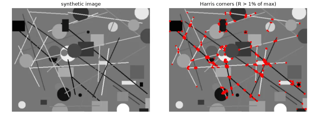

A synthetic test image and its Harris corners: the responses sit where lines cross and at the corners of rectangles, not along straight edges or inside flat shapes

Harris doesn’t care about rotation (eigenvalues don’t change when you rotate), but it does care about scale: a corner at one zoom level can look like a smooth curve at another.

SIFT: handling scale, plus a gradient-histogram descriptor

Lowe’s SIFT adds scale. It blurs the image with Gaussians of growing $\sigma$ and subtracts neighbouring levels. That gives a Difference-of-Gaussians (DoG) stack, which is a cheap stand-in for the scale-normalised Laplacian. Keypoints are local extrema in $x$ , $y$ and scale, so each one comes with its own natural size. Low-contrast points and points on edges get thrown out.

Next, each keypoint gets a dominant orientation from a histogram of gradient directions around it. The descriptor is computed in a patch rotated to that orientation and scaled to the keypoint’s size: a $4 \times 4$ grid of cells, each with an 8-bin histogram of gradient orientations, so $4 \times 4 \times 8 = 128$ numbers. The vector is normalised (then clipped at 0.2 and normalised again) so lighting changes matter less. So basically you get something that doesn’t change with rotation or scale and copes OK with moderate changes in viewpoint and lighting. The patent ran out in 2020, and SIFT is now in the main OpenCV package.

ORB: fast binary features

ORB was made as a free, fast alternative. It finds corners with FAST: a pixel counts as a corner if a long enough arc of the 16 pixels on a circle around it is all brighter or all darker. It ranks them with the Harris score and uses an image pyramid to handle scale. The orientation comes from the intensity centroid of the patch (roughly, the “centre of brightness”). The descriptor is rotated BRIEF: 256 yes/no tests like “is pixel $p$ brighter than pixel $q$ ?” on a smoothed patch, stored as 32 bytes. Comparing two binary descriptors is just an XOR and a bit count, which is much faster than a distance between two 128-D float vectors.

Matching descriptors

For each descriptor in image 1, find the closest descriptor in image 2. Pick the right distance:

L2 (Euclidean) for float descriptors like SIFT;
Hamming (how many bits differ) for binary descriptors like ORB, BRIEF and AKAZE.

Plain nearest-neighbour matching gives lots of wrong matches, because every descriptor gets a partner, even when its real partner isn’t visible in the other image. Two common filters:

Lowe’s ratio test: find the two nearest neighbours and keep the match only if $d_1 < r\,d_2$ , with $r$ around 0.7–0.8. The idea is that a correct match is usually much closer than the runner-up. An ambiguous one (say, on repeated texture) isn’t.
Cross-check: keep a match only if $a$ ‘s nearest neighbour is $b$ and $b$ ‘s nearest neighbour is $a$ .

def ratio_matches(d1, d2, norm, ratio=0.75):
    bf = cv2.BFMatcher(norm)                 # cv2.NORM_L2 for SIFT, cv2.NORM_HAMMING for ORB
    good = []
    for m, n in bf.knnMatch(d1, d2, k=2):
        if m.distance < ratio * n.distance:  # best clearly better than second best
            good.append(m)
    return good

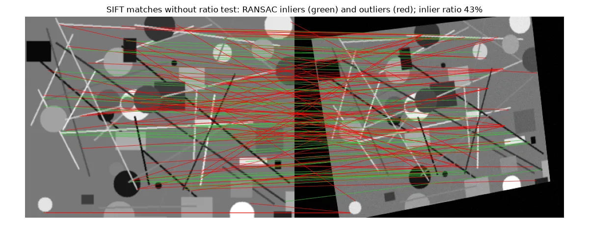
On the synthetic pair (the second image is the first one warped by a known homography, plus noise), I counted how many matches were really correct, meaning within 3 pixels of where the known homography sends the point:

Matches	Count	Correct
SIFT, plain nearest neighbour	1082	43%
SIFT, ratio test 0.75	440	86%
ORB, ratio test 0.8	489	92%

The ratio test throws away more than half the matches, but most of what it throws away is wrong. Still, even 10% bad matches would wreck a least-squares fit. That’s where RANSAC comes in.

RANSAC

RANdom SAmple Consensus (Fischler and Bolles, 1981) fits a model to data with lots of outliers (points that just don’t fit). The steps:

Pick a minimal sample at random: 4 matches for a homography (see the geometric transformations note for why 4).
Fit the model to that sample exactly (the DLT).
Count inliers: matches whose reprojection error $\lVert \mathbf{H}\mathbf{p}_i - \mathbf{q}_i \rVert$ is under a threshold, usually 1–5 pixels.
Repeat, keep the model with the most inliers, and at the end refit it on all of its inliers with least squares.

def ransac_homography(src, dst, thresh=3.0, iters=2000, rng=np.random.default_rng(0)):
    best = np.zeros(len(src), bool)
    for _ in range(iters):
        idx = rng.choice(len(src), 4, replace=False)         # minimal sample
        H = dlt(src[idx], dst[idx])                          # exact fit to 4 pairs
        err = np.linalg.norm(project(H, src) - dst, axis=1)  # reprojection error
        inliers = err < thresh
        if inliers.sum() > best.sum():
            best = inliers
    return dlt(src[best], dst[best]), best                   # refit on all inliers

Here dlt is the homography_dlt solver from the geometric transformations note (exact for 4 pairs, least squares for more), and project applies $\mathbf{H}$ and divides by the third coordinate. How many iterations do you need? If a fraction $w$ of the matches are inliers, a random sample of $s$ matches is all inliers with probability $w^s$ . To get at least one clean sample with probability $p$ , you need

N = \frac{\log(1 - p)}{\log(1 - w^s)}.

With $p = 0.99$ and $s = 4$ : $w = 0.9$ needs 5 iterations, $w = 0.5$ needs 72, $w = 0.3$ needs 567, and $w = 0.1$ needs about 46,000. This is the part that made it click for me: the cost blows up as inliers get rare, so cleaning the matches with the ratio test first really pays off. Real implementations usually update $N$ as they go, using the best inlier ratio found so far.

To push it, I gave RANSAC the plain nearest-neighbour SIFT matches, where only 43% were correct. It still found the right model:

H_true                     H_RANSAC (own)              H_RANSAC (OpenCV)
[ 0.9     0.15   30.  ]    [ 0.8989  0.1488  30.27]    [ 0.8995  0.1505  30.04]
[-0.1     0.95   40.  ]    [-0.0999  0.9483  40.22]    [-0.1007  0.9509  40.09]
[ 0.0002  0.0001  1.  ]    [ 0.0002  0.0001   1.  ]    [ 0.0002  0.0001   1.  ]

On average, the true and estimated mappings disagreed by 0.15 pixels over the image. OpenCV’s findHomography(src, dst, cv2.RANSAC, 3.0) gives almost the same thing. It also normalises the points and polishes the final model with Levenberg–Marquardt, which is why it lands a little closer.

SIFT matches without the ratio test between the synthetic image and its warped copy, with RANSAC inliers in green and outliers in red

Warping one image onto the other

Once you have $\mathbf{H}$ , cv2.warpPerspective(img1, H, (w, h)) resamples image 1 into image 2’s frame (by inverse mapping, as in the geometric transformations note). In the test, the mean absolute difference between the warped image and the target inside the overlap was 3.5 grey levels, which is close to the noise I added.

Two limits to remember. First, one homography is only right for a flat scene or a camera that only rotates. For a 3D scene seen from two places you need the fundamental or essential matrix, which is also estimated with RANSAC. Second, RANSAC fails when inliers are very rare, or when a wrong model gets more support than the right one, for example with strongly repeated texture. Variants like PROSAC (which tries good matches first), LO-RANSAC, MAGSAC and OpenCV’s USAC_MAGSAC flag are meant for these cases. Learned detectors and matchers (SuperPoint, LightGlue, LoFTR) now replace hand-made features in hard conditions, but the RANSAC step usually stays.

Key takeaways

Corners make good keypoints because the brightness changes in two directions. The Harris score measures that using the eigenvalues of the structure tensor.
SIFT adds scale (DoG extrema) and a 128-D gradient-histogram descriptor. ORB is a fast binary alternative built on FAST and rotated BRIEF.
Match float descriptors with L2 and binary ones with Hamming distance, then filter with the ratio test or cross-check.
RANSAC fits a homography from random 4-point samples and keeps the one with the most inliers. The number of iterations needed grows fast as the inlier ratio drops.
Always refit on all the inliers at the end, and remember that one homography only fits a plane or a pure rotation.

Resources

David G. Lowe, Distinctive Image Features from Scale-Invariant Keypoints, IJCV 60(2), 2004.
Ethan Rublee, Vincent Rabaud, Kurt Konolige and Gary Bradski, ORB: An efficient alternative to SIFT or SURF, ICCV 2011.
Chris Harris and Mike Stephens, A Combined Corner and Edge Detector, Alvey Vision Conference, 1988.
Martin A. Fischler and Robert C. Bolles, Random Sample Consensus, Communications of the ACM 24(6), 1981.
Richard Szeliski, Computer Vision: Algorithms and Applications, 2nd ed., 2022: Chapter 7 and Section 8.1.
Richard Hartley and Andrew Zisserman, Multiple View Geometry in Computer Vision, 2nd ed., 2004: Section 4.7 (robust estimation).
OpenCV feature detection and description tutorials and the findHomography documentation.
Related notes: 2D geometric transformations and homographies, linear filters and the Gaussian blur.