YOLOv1: object detection as one regression on a grid

Before YOLO, the best detectors worked in two stages. First they proposed a few thousand candidate regions, then they classified each one. That’s accurate but slow: R-CNN ran the network once for every region, and even the faster versions still had a separate, slow proposal step. YOLOv1 (2015) asked a simpler question: can one network look at the whole image once and directly spit out every box and its class? It turned out yes, at 45 frames per second. Almost every real-time detector today still uses the idea it started: a grid of cells, where each cell predicts boxes from the features at its spot.

The grid idea

YOLOv1 resizes the image to 448×448 and cuts it into an $S \times S$ grid, with $S = 7$ . Each object belongs to exactly one cell: the cell that has the centre of its box. That cell is “responsible” for the object. Every other cell has to learn to say “nothing here”.

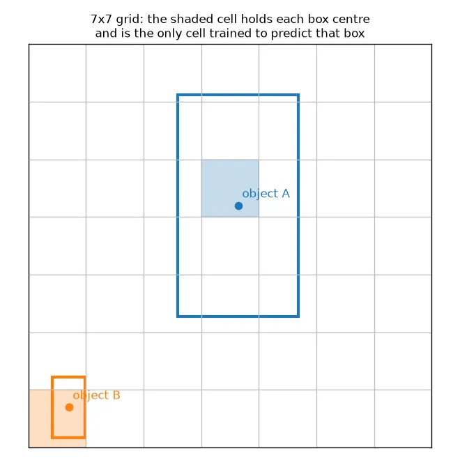
A 7x7 grid over an image. Two boxes are drawn; the cell containing each box centre is shaded, showing which cell is responsible for that object.

Each cell predicts:

$B$ boxes (the paper uses $B = 2$ ). Each box has five numbers: $x, y, w, h$ and a confidence.
$C$ class probabilities (20 for Pascal VOC), shared by the cell’s boxes.

So the whole output is one tensor of shape $S \times S \times (5B + C) = 7 \times 7 \times 30$ . That’s the bit that made it click for me: detection has turned into regression. The network just fills a fixed-size tensor, and the loss compares it with a target tensor laid out the same way.

The coordinates are set up so every number stays in a small, predictable range:

$x, y$ are the box centre relative to the cell, in $[0, 1)$ . So $(0.5, 0.5)$ means the middle of the cell.
$w, h$ are the box width and height relative to the whole image, in $[0, 1]$ .
The confidence is trained towards $P(\text{object}) \times \text{IoU}(\text{pred}, \text{truth})$ . It’s zero for empty cells, and for the responsible box it equals the IoU (overlap) between the predicted box and the real one.

Packing the labels into the grid

Labels usually come as normalised $(c_x, c_y, w, h)$ boxes per image (the “YOLO format”). Turning them into the grid target only takes a few lines:

import torch

S, B, C = 7, 2, 20          # grid size, boxes per cell, classes

def encode_target(boxes, S=7, C=20):
    """boxes: list of (class_id, cx, cy, w, h), all normalised to [0, 1]."""
    target = torch.zeros(S, S, C + 5)
    for cls, cx, cy, w, h in boxes:
        row, col = int(cy * S), int(cx * S)          # cell that holds the centre
        x_cell, y_cell = cx * S - col, cy * S - row  # centre offset inside that cell, in [0, 1)
        if target[row, col, C] == 0:                 # one object per cell in YOLOv1
            target[row, col, cls] = 1.0              # one-hot class
            target[row, col, C] = 1.0                # "an object lives here"
            target[row, col, C+1:C+5] = torch.tensor([x_cell, y_cell, w, h])
    return target

t = encode_target([(11, 0.52, 0.40, 0.30, 0.55), (14, 0.10, 0.90, 0.08, 0.15)])
print(t.shape)                       # torch.Size([7, 7, 25])
print(t[..., C].nonzero().tolist())  # [[2, 3], [6, 0]]: cells that own an object

The target only stores one box per cell, but the prediction has $B = 2$ . This confused me at first. During training, whichever predicted box has the higher IoU with the real box becomes the responsible one. Over time the two box slots specialise, each getting better at certain sizes and shapes of object.

Look at the if line. If two object centres land in the same cell, the second one just gets dropped. That’s a real limit of YOLOv1, not a shortcut in my code.

The network

The backbone is a stack of 24 convolutional layers, inspired by GoogLeNet. It switches between $1\times1$ “reduction” convolutions (they shrink the number of channels) and $3\times3$ convolutions, and ends with two fully connected layers. The last layer gives $7 \cdot 7 \cdot 30 = 1470$ numbers, which get reshaped into the grid. Since the head is fully connected, each cell’s prediction can use information from the whole image. Later YOLO versions swapped the fully connected head for convolutions (see dense detection heads).

The loss, one piece at a time

Everything is trained with sum-squared error, but with weights that fix three problems. Let $\mathbb{1}_{ij}^{\text{obj}}$ be 1 when box $j$ of cell $i$ is responsible for an object, and $\mathbb{1}_{ij}^{\text{noobj}}$ be 1 otherwise. Hats mark predictions.

\begin{aligned} \mathcal{L} = {} & \lambda_{\text{coord}} \sum_{i,j} \mathbb{1}_{ij}^{\text{obj}} \left[(x_i - \hat{x}_i)^2 + (y_i - \hat{y}_i)^2\right] \\ & + \lambda_{\text{coord}} \sum_{i,j} \mathbb{1}_{ij}^{\text{obj}} \left[\left(\sqrt{w_i} - \sqrt{\hat{w}_i}\right)^2 + \left(\sqrt{h_i} - \sqrt{\hat{h}_i}\right)^2\right] \\ & + \sum_{i,j} \mathbb{1}_{ij}^{\text{obj}} (C_i - \hat{C}_i)^2 + \lambda_{\text{noobj}} \sum_{i,j} \mathbb{1}_{ij}^{\text{noobj}} (C_i - \hat{C}_i)^2 \\ & + \sum_{i} \mathbb{1}_{i}^{\text{obj}} \sum_{c} \left(p_i(c) - \hat{p}_i(c)\right)^2 \end{aligned}

Here $C_i$ is the confidence, $p_i(c)$ the probability of class $c$ , and $\mathbb{1}_i^{\text{obj}}$ is 1 if any object’s centre is in cell $i$ .

Empty cells are the vast majority. In a normal image only a few of the 98 box slots hold an object. Their confidence errors would drown out everything else and push all confidences to zero. So the “no object” term is turned down with $\lambda_{\text{noobj}} = 0.5$ .
Box position needs more weight. Coordinate errors are turned up with $\lambda_{\text{coord}} = 5$ , so the network doesn’t give up box quality for classification.
Big and small boxes aren’t the same. A 10-pixel error is a disaster for a 20-pixel box and nothing for a 400-pixel one. Taking the square root of $w$ and $h$ before the squared error makes the same error in pixels cost more for small boxes.

In code, the square root of a raw network output needs care, because early in training $w$ can be negative. A common trick is $\text{sign}(w)\sqrt{|w| + \epsilon}$ , which keeps the gradient finite and the sign the same. Many implementations, including the one I followed, also use 1 instead of the IoU as the confidence target. That’s a simplification of the paper, and it works fine in practice.

Turning the grid back into boxes

At test time each cell gives $B$ boxes. A box’s score for a class is its confidence times the cell’s class probability. Getting back to image coordinates is just the encoding in reverse:

def decode(pred, S=7, C=20, B=2):
    """pred: (S, S, C + 5B) raw network output for one image -> list of boxes."""
    out = []
    for row in range(S):
        for col in range(S):
            cell = pred[row, col]
            cls_prob = cell[:C]
            for b in range(B):
                conf, x, y, w, h = cell[C + 5*b : C + 5*b + 5]
                score = conf * cls_prob.max()          # class-specific confidence
                cx, cy = (col + x) / S, (row + y) / S  # back to image coordinates
                out.append((int(cls_prob.argmax()), float(score), float(cx), float(cy), float(w), float(h)))
    return out

torch.manual_seed(0)
print(len(decode(torch.rand(S, S, C + 5*B))))   # 98 candidate boxes

That gives $7 \times 7 \times 2 = 98$ candidates. Low-score boxes are thrown away, and non-maximum suppression (NMS) removes duplicates, for example when neighbouring cells both found the same large object. The final detections are then scored with mean average precision (see mAP).

What it’s good at, and where it struggles

YOLOv1 was very fast, and it made fewer background false positives than Fast R-CNN, because it sees the whole image as context. Its weak spots all come from the coarse grid:

Crowds of small objects. Each cell can predict at most $B$ boxes and only one class. A flock of birds in one cell mostly gets lost.
Rough box positions. Boxes are predicted from a 7×7 grid after a lot of downsampling, so they’re less precise than two-stage detectors.
Odd aspect ratios. Box shapes are learned from scratch, with no starting guess. YOLOv2 fixed this by adding anchor boxes (see anchors and designing anchors), and YOLOv3 added predictions at three scales.

Key takeaways

YOLOv1 does detection by filling one $S \times S \times (5B + C)$ tensor in a single forward pass.
The cell that holds an object’s centre is responsible for it. Box centres are stored relative to that cell, sizes relative to the image.
The loss is plain squared error with three fixes: turn down empty cells, turn up coordinates, and use $\sqrt{w}, \sqrt{h}$ so small boxes count.
The grid only allows a few objects per cell, which hurts with small, crowded objects. Anchors and multi-scale heads in later versions deal with this.

Resources

Redmon, Divvala, Girshick, Farhadi, “You Only Look Once: Unified, Real-Time Object Detection”, CVPR 2016. arXiv:1506.02640
Aladdin Persson, “YOLOv1 from scratch” video and the Machine-Learning-Collection repo. I coded along with it; the snippets above are my own rewrites.
Pascal VOC dataset: host.robots.ox.ac.uk/pascal/VOC
Related notes: anchors and RPNs, dense detection heads, mean average precision, overlap-based losses.