Class activation maps: CAM and Grad-CAM

A classifier only tells you what is in an image. A lot of the time you also want to know where it saw it. Maybe the model is cheating by looking at the background, maybe you want to explain a prediction, or maybe you want rough object locations without paying for box labels. Class activation maps (CAM) give you this almost for free. They reuse the classifier’s own weights to paint a heatmap over the image, one map per class. Grad-CAM takes the same idea and makes it work on any convolutional network, not just ones that end in a special way.

What the network has to look like for CAM

CAM was made for networks that end like this:

convolutional layers that produce $K$ feature maps $f_k(x, y)$ of size $h \times w$ ,
global average pooling (GAP), which turns each map into one number $F_k = \frac{1}{hw}\sum_{x,y} f_k(x,y)$ ,
one linear layer that gives the score (logit) of each class $c$ : $S_c = \sum_k w_k^c F_k$ .

GAP became popular with Network In Network, as a replacement for the big fully connected layers at the end of networks like VGG. It has no parameters, it works for any input size, and it pushes each channel to act like a “detector” where only its overall strength matters.

Pushing the weights back onto the map

Here’s the trick. Put the GAP formula into the score and swap the order of the two sums:

S_c = \sum_k w_k^c \frac{1}{hw}\sum_{x,y} f_k(x,y) = \frac{1}{hw}\sum_{x,y} \underbrace{\sum_k w_k^c f_k(x,y)}_{M_c(x,y)}

Here $w_k^c$ is the weight that connects channel $k$ to class $c$ , and $M_c(x,y)$ is the class activation map. It’s just a weighted sum of the feature maps, using that class’s weights. So basically: the class score is the average of $M_c$ over all positions, which means $M_c(x, y)$ tells you how much the spot $(x,y)$ adds to the decision for class $c$ . I liked that nothing extra gets trained here. The map just falls out of the classifier you already have.

The last feature map is smaller than the input (by the network’s total stride), so you upsample $M_c$ to the image size, normalise it, and lay it over the image as a heatmap.

A tiny example you can run

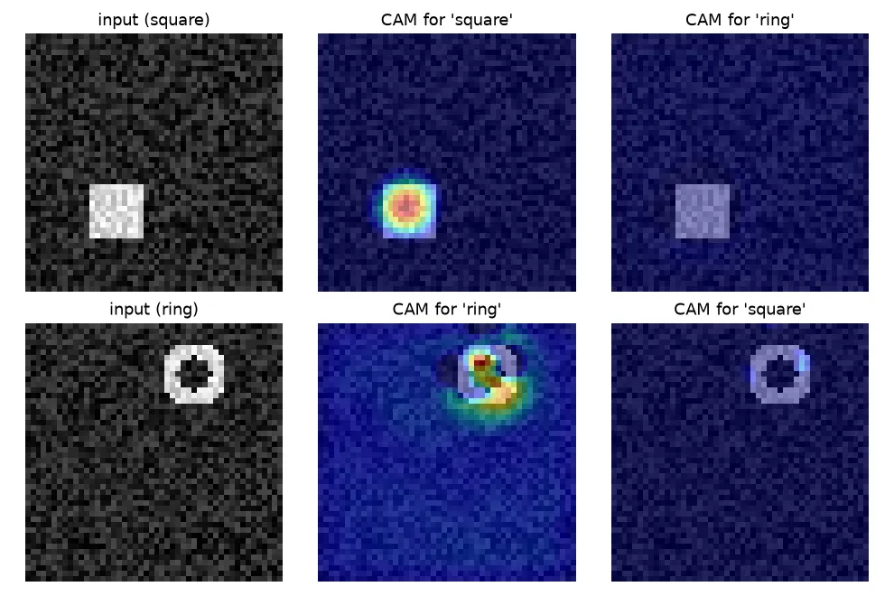
To keep it self-contained, here’s a small network trained on made-up images: noise with either a bright square (class “square”) or a bright ring (class “ring”) somewhere random. It gets to 100% accuracy within a few hundred steps on a CPU.

import torch, torch.nn as nn, torch.nn.functional as F

class TinyCAMNet(nn.Module):
    def __init__(self, n_classes=2):
        super().__init__()
        self.features = nn.Sequential(            # total stride 2: 48x48 -> 24x24
            nn.Conv2d(1, 16, 3, padding=1), nn.ReLU(), nn.MaxPool2d(2),
            nn.Conv2d(16, 32, 3, padding=1), nn.ReLU(),
            nn.Conv2d(32, 32, 3, padding=1), nn.ReLU())
        self.fc = nn.Linear(32, n_classes)        # used after global average pooling

    def forward(self, x):
        f = self.features(x)                      # (B, K, h, w)
        return self.fc(f.mean(dim=(2, 3))), f     # logits, feature maps

def cam(model, x, c):
    _, f = model(x)
    w = model.fc.weight[c]                        # (K,) weights for class c
    return torch.einsum("k,khw->hw", w, f[0]).detach()

The figure shows what you get after training. For the square, the “square” map lights up the whole square, and the “ring” map stays dark. For the ring, the map is strongest on only part of the ring. That’s normal. CAM highlights the parts that tell the classes apart, and that isn’t always the whole object.

Synthetic images of a square and a ring in noise, each overlaid with the CAM for its own class (bright on the object) and for the other class (dark)

Why average pooling and not max pooling

The CAM paper compared GAP with global max pooling (GMP) and found GAP finds objects better. You can see why from the gradients. With GAP, every position adds to the pooled value, so training pushes the network to respond over the whole object. With GMP, only the single strongest position counts, so the network only needs one good spot.

f = torch.rand(1, 1, 4, 4, requires_grad=True)   # one 4x4 feature map
f.mean().backward()                               # GAP
print((f.grad > 0).sum().item())                  # 16: every position gets gradient
f.grad = None
f.amax().backward()                               # GMP
print((f.grad > 0).sum().item())                  # 1: only the max position

Both get about the same classification accuracy. The difference is how much of the object the maps cover.

How sharp the map can be

The map can only be as sharp as the last feature map. A $7 \times 7$ map for a $224 \times 224$ image means each cell covers 32 pixels, so the upsampled heatmap looks blobby. The CAM authors got better localisation by cutting off the last few layers of VGG or GoogLeNet so the final conv map was bigger (about $14 \times 14$ ), then adding a new conv layer, GAP and a linear layer, and fine-tuning. They called this the mapping resolution. The catch is that shallower features understand less about what things are. If you want to see what different depths of a backbone look like, see Tapping a CNN backbone.

Grad-CAM: getting the weights from gradients

The weak spot of CAM is that architecture rule. Most networks don’t end in GAP plus one linear layer, and you don’t want to retrain them. Grad-CAM gets rid of the rule. For any differentiable model and any conv layer with feature maps $A_k$ , it says the importance of channel $k$ for class $c$ is the average gradient of the class score with respect to that channel:

\alpha_k^c = \frac{1}{hw}\sum_{x,y} \frac{\partial S_c}{\partial A_k(x,y)}, \qquad L^c_{\text{Grad-CAM}} = \mathrm{ReLU}\Big(\sum_k \alpha_k^c A_k\Big)

The ReLU keeps only the regions that push the score up. Use the score before softmax (the logit). After softmax, one class can go up just because others went down, and that makes the gradients messy.

def grad_cam(model, x, c):
    logits, f = model(x)
    f.retain_grad()                         # keep the gradient of a non-leaf tensor
    logits[0, c].backward()                 # d(score_c) / d(feature maps)
    alpha = f.grad[0].mean(dim=(1, 2))      # one weight per channel
    return F.relu(torch.einsum("k,khw->hw", alpha, f[0])).detach()

The nice part: for a GAP-plus-linear network, the two methods give the same answer. The gradient of $S_c$ with respect to $f_k(x,y)$ is $w_k^c / (hw)$ at every position, so $\alpha_k^c = w_k^c/(hw)$ , and Grad-CAM is exactly $\mathrm{ReLU}(M_c)/(hw)$ . On the tiny model above, torch.allclose(grad_cam(m, x, c), F.relu(cam(m, x, c)) / (h * w)) returns True. So CAM is really just a special case of Grad-CAM.

In a pretrained network you usually pick the last convolutional layer. Its features know the most about what things are, and they still keep a spatial layout. Earlier layers give sharper maps that care less about the class. In Keras or PyTorch the practical step is the same: build a model (or use a hook) that gives you both that layer’s activations and the logits, then take the gradient.

What CAMs can and can’t tell you

They’re coarse. They show regions, not exact object edges.
They show what the model is using, not what’s “correct”. If a classifier learned that boats come with water, the CAM will light up the water. That’s exactly why they’re handy for debugging.
You can turn them into rough boxes by thresholding the map (the CAM paper kept the biggest connected region above 20% of the max). A lot of weakly supervised localisation methods (finding objects without box labels) build on this. It also inspired counting models that read a heatmap out of a network trained only on a count. See Density maps for counting.

Key takeaways

With GAP followed by one linear layer, the class score is the average over space of $M_c = \sum_k w_k^c f_k$ , so $M_c$ is a free map of where the evidence is.
GAP gives better maps than global max pooling, because every location gets gradient during training, not just the peak.
The map can’t be sharper than the last feature map (the mapping resolution).
Grad-CAM gets the channel weights from averaged gradients, works on any CNN, and turns into CAM (up to a constant) for GAP-plus-linear heads.
Use logits, not softmax outputs, and usually the last conv layer.

Resources

Zhou, Khosla, Lapedriza, Oliva, Torralba, Learning Deep Features for Discriminative Localization, CVPR 2016. The CAM paper, including GAP vs GMP and mapping resolution.
Selvaraju et al., Grad-CAM: Visual Explanations from Deep Networks via Gradient-based Localization, ICCV 2017.
Lin, Chen, Yan, Network In Network, 2013. Introduces global average pooling as a classifier head.
François Chollet, Grad-CAM class activation visualization, Keras code examples. The Keras recipe I first followed with a pretrained VGG16.