Counting dense objects with density and confidence maps

When objects are tiny and packed together (people in a stadium, cells under a microscope, birds in a flock), box detectors have a hard time. The boxes overlap so much that non-max suppression throws away real objects, and drawing hundreds of boxes per image by hand is slow. There’s a simpler idea that works better: mark each object with a single point, turn those points into a smooth map, and train a fully convolutional network to predict that map. Then you read the count, and often the positions, back out of the prediction. These notes cover how the target maps are built and how to decode them.

Two kinds of target map

Both start from point labels $p_1, \dots, p_N$ and put a 2D Gaussian blob $G_\sigma$ on each point. The difference is how the blobs are combined.

A density map adds up blobs that each have a total mass of one:

D(x) = \sum_{i=1}^{N} G_{\sigma_i}(x - p_i), \qquad \int G_\sigma = 1 \;\Rightarrow\; \sum_x D(x) = N

Here $x$ is a pixel position and $\sigma_i$ is how wide the blob for object $i$ is. So basically, if you add up the map over any region, you get the number of objects in that region. Counting is just summing the predicted map. This idea goes back to Lempitsky and Zisserman (2010) and is the usual target in crowd counting.

A confidence map uses blobs whose peak is 1 and combines them with a maximum instead of a sum:

C(x) = \max_i \exp\!\Big(-\frac{\lVert x - p_i\rVert^2}{2\sigma^2}\Big)

Now each pixel means “how likely is an object centre here”, which fits a sigmoid output nicely. Its sum is not the count. You count by finding peaks instead. The MSS paper (de Arruda et al., 2021) uses this kind of map so it can return positions, not just a number.

import numpy as np

def kernel_at(x, y, sigma, shape):
    yy, xx = np.mgrid[:shape[0], :shape[1]]
    return np.exp(-((xx - x)**2 + (yy - y)**2) / (2 * sigma**2))

def density_map(points, shape, sigma):
    d = np.zeros(shape)
    for x, y in points:
        g = kernel_at(x, y, sigma, shape)
        d += g / g.sum()        # normalize inside the image so edge objects still count as 1
    return d

def confidence_map(points, shape, sigma):
    c = np.zeros(shape)
    for x, y in points:
        c = np.maximum(c, kernel_at(x, y, sigma, shape))   # peak 1, overlaps do not add up
    return c

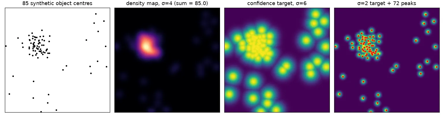
On 85 synthetic points in a $128 \times 128$ image, density_map(...).sum() gives 85.0. The common shortcut, putting a 1 at each point and calling gaussian_filter(..., mode="constant"), gave 83.6 on the same points. The reason is that blobs near the border lose the part that falls outside the image. Renormalizing each blob (or using a reflecting border) fixes it.

Synthetic object centres, their density map whose sum equals the count, a wide confidence target, and a narrow confidence target with detected peaks marked in red

Picking sigma

How wide the blob is ( $\sigma$ ) is the main choice you make.

Fixed $\sigma$ . Simple, and fine when all objects are about the same size in pixels (a top-down view at a constant scale, or cells at a fixed magnification).
Size-based $\sigma$ . If you have box sizes, tie $\sigma$ to the object size, for example a fraction of the box diagonal.
Geometry-adaptive $\sigma$ . With perspective, nearby objects look bigger and far ones look smaller and more crowded. The multi-column CNN paper (Zhang et al., 2016) sets $\sigma_i = \beta \bar d_i$ , where $\bar d_i$ is the average distance from point $i$ to its $k$ nearest neighbours, with $\beta \approx 0.3$ and $k = 3$ . Crowded areas get narrow blobs and sparse areas get wide ones. Clip it to a sensible minimum, because two almost identical points give $\sigma \approx 0$ .

from scipy.spatial import cKDTree

def adaptive_sigmas(points, k=3, beta=0.3, min_sigma=1.0):
    dist, _ = cKDTree(points).query(points, k=k + 1)   # column 0 is the point itself
    return np.maximum(beta * dist[:, 1:].mean(1), min_sigma)

If $\sigma$ is too small, the network gets a spiky target that’s almost impossible to hit. If it’s too large, neighbouring objects blur into one blob. That doesn’t hurt the density sum, but it ruins finding objects by their peaks.

Matching the network’s output size

A backbone usually predicts the map at a lower resolution, for example $1/8$ of the input. So the target has to be shrunk to that size without changing its sum. This tripped me up: normal bilinear resizing doesn’t keep the sum. Shrinking by 8 in each direction divides it by about 64. Sum-pooling does keep it:

def sum_pool(d, s):
    h, w = d.shape[0] // s, d.shape[1] // s
    return d[:h*s, :w*s].reshape(h, s, w, s).sum(axis=(1, 3))

The other option is to build the target straight at the output resolution, by dividing the point coordinates and $\sigma$ by the stride. For confidence maps the sum doesn’t matter, so you can build them at low resolution directly. Just remember to multiply the found positions back by the stride.

Getting the count and positions back

Summing. For a density map, the predicted count is $\hat N = \sum_x \hat D(x)$ . It’s stable, copes with heavy overlap, and needs no threshold. But it gives no positions, and a model can land on the right total for the wrong reasons.

Peak finding. For a confidence map, an object is a pixel that’s a local maximum and above a threshold $\tau$ . The MSS paper checks the 4 direct neighbours and uses $\tau = 0.35$ . A $3 \times 3$ maximum filter does the same job:

from scipy.ndimage import maximum_filter

def find_peaks(conf, tau=0.35):
    is_max = conf == maximum_filter(conf, size=3)   # local maximum in a 3x3 window
    ys, xs = np.nonzero(is_max & (conf > tau))
    return np.stack([xs, ys], 1)

The way I think about it, this is the map version of non-max suppression: a peak wins over its neighbours. Its weak spot shows up in the figure. On the ideal $\sigma = 2$ target it finds 72 of the 85 objects, because centres closer than a couple of pixels merge into one peak. Narrower targets, a higher output resolution, or a smaller minimum distance between peaks all help. Summing doesn’t have this problem, so some systems report the sum as the count and use peaks only for locations.

Models built around these maps

Context with pyramid pooling. Whether a small blob is an object often depends on what’s around it. The MSS model adds a pyramid pooling module (from PSPNet) after a VGG-style backbone. It pools the feature map into $1\times1$ , $2\times2$ , $3\times3$ and $6\times6$ grids, runs a $1\times1$ convolution on each, upsamples them back, and concatenates them with the original features. That way every pixel gets a summary of the whole image and of its own area (crowded or sparse). (More on this in spatial pyramid pooling.)

Multi-sigma refinement. Instead of one output, the MSS model predicts $T$ confidence maps in stages. Each stage sees the features plus the previous stage’s map. The targets get sharper at each stage: stage 1 uses $\sigma_{\max}$ , the last stage uses $\sigma_{\min}$ , and the ones in between use evenly spaced values. Early stages learn the easy question “roughly where are the objects?” and later stages narrow it down to exact centres. It’s the same coarse-to-fine idea used in multi-stage pose estimators. Only the last map gets decoded.

Heatmap regulation. Aich and Stavness start from the simplest counter: a backbone, global average pooling (GAP) and one linear output that predicts the count directly. A model like that can learn to hit the right number while looking at the wrong places, for example counting some background to make up for objects it missed. Their fix: take the class activation map that the GAP head already gives you (see class activation maps), and add a loss that pulls it towards a Gaussian map built from the point labels. The count head stays the same, but now it has to base its answer on the actual objects.

Perspective-aware maps. For crowds seen from an angle, Zhang et al. (2015) built the density target from a head blob plus a body blob, scaled by a perspective map, because people aren’t circles and their size changes with distance. The general lesson I took from this: the target blob should match what one object actually looks like in the image.

Key takeaways

Point labels plus a predicted map are a practical alternative to boxes when objects are small, many and overlapping.
A density map (blobs with mass 1, added up) gives the count by summing. A confidence map (blobs with peak 1, combined by max) gives positions by finding peaks.
Pick $\sigma$ to match how big an object looks: fixed, size-based, or adaptive from nearest-neighbour distances.
Keep the count exact: renormalize blobs at image borders and shrink density targets with sum-pooling, not resizing.
Context (pyramid pooling), coarse-to-fine targets (multi-sigma stages) and checking where the model looks (heatmap regulation) all help dense counting.

Resources

Lempitsky and Zisserman, Learning To Count Objects in Images, NeurIPS 2010. The density-map formulation.
Zhang et al., Single-Image Crowd Counting via Multi-Column CNN, CVPR 2016. Geometry-adaptive kernels.
Zhang et al., Cross-scene Crowd Counting via Deep Convolutional Neural Networks, CVPR 2015. Perspective-normalized density maps.
de Arruda et al., Counting and locating high-density objects using convolutional neural network, 2021. Pyramid pooling, multi-sigma refinement and peak-based localization.
Aich and Stavness, Improving Object Counting with Heatmap Regulation, 2018.
Zhao et al., Pyramid Scene Parsing Network, CVPR 2017. The pyramid pooling module.