Overlapping polygons at scale: find pairs with an STRtree, then split the overlaps

Detection and segmentation models predict objects one at a time, so neighbouring polygons often overlap: two crowns claiming the same leaves, two buildings sharing a wall. Before you can count, measure or export the polygons, every overlap needs an owner. Step one is finding which polygons overlap at all. The obvious double loop works fine for a few hundred polygons, but with tens of thousands the way you search decides whether this takes milliseconds or minutes. So here’s how a spatial index makes the search fast, and two ways to split what you find. (Fixing invalid polygons first is in polygon validity and shape metrics.)

Why checking every pair is too slow

The obvious approach tests every polygon against every other one: $n(n-1)/2$ tests. Double the number of polygons and the work goes up four times. That’s $O(n^2)$, and each test isn’t free either, since an exact intersects on two polygons with $v$ vertices costs more than comparing two boxes.

But almost all of those tests are pointless. A polygon in one corner of the map can’t touch one in the other corner. What we want is a way to ask “which polygons are near this one?” without looking at all of them.

The idea behind an STRtree

An R-tree groups nearby objects into boxes, then groups those boxes into bigger boxes, and so on up to one root box. Each node only stores the bounding box of what’s below it. To find everything that might touch a query shape, you start at the root and only go down into boxes that overlap the query’s box. So whole regions of the map get skipped with one comparison.

An STRtree (Sort-Tile-Recursive) is an R-tree built in one go from a fixed set of geometries. It sorts the boxes by $x$, cuts them into vertical slices, sorts each slice by $y$, and packs neighbours into full nodes. Building it costs $O(n \log n)$ (that’s the sorting). A query costs about $O(\log n + k)$, where $k$ is the number of boxes it returns. So querying all $n$ polygons costs about $O(n \log n + K)$, with $K$ the total number of candidate pairs. That’s close to $O(n)$ times the usual number of neighbours, as long as the density doesn’t grow with the map.

The search has two phases:

1. Filter: the tree returns candidates whose bounding boxes intersect the query box. Cheap, but it includes false alarms (two round crowns can have touching boxes and still not touch).
2. Refine: an exact geometric test (intersects, overlaps, …) runs on the candidates only.

In Shapely 2, both phases happen in one vectorised call:

import numpy as np, shapely
from shapely.strtree import STRtree

def random_crowns(n, seed=0):
    rng = np.random.default_rng(seed)
    side = np.sqrt(n) * 10                                 # constant density as n grows
    pts = shapely.points(rng.uniform(0, side, (n, 2)))
    return shapely.buffer(pts, rng.uniform(2, 5, n))       # discs with radius 2-5

def overlapping_pairs(geoms):
    tree = STRtree(geoms)
    i, j = tree.query(geoms, predicate="intersects")       # filter + refine, all at once
    keep = i < j                                           # drop self-pairs and (j, i) duplicates
    return i[keep], j[keep]

geoms = random_crowns(4000)
i, j = overlapping_pairs(geoms)

Passing an array to query gives back a $2 \times m$ array: row 0 indexes the input, row 1 the tree. Every polygon intersects itself, so the pairs $(k, k)$ are always there, and each real pair shows up twice. i < j gets rid of both. In GeoPandas the same call is gdf.sindex.query(gdf.geometry, predicate="intersects"), or a self spatial join with gpd.sjoin(gdf, gdf, predicate="intersects").

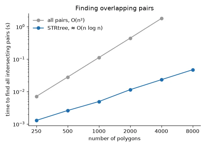
On random discs, the all-pairs loop takes 1.8 s for 4,000 polygons. The tree takes 0.02 s and finds the same pairs. And the gap keeps growing, because it’s a different growth rate, not just a constant speed-up.

Two bugs that look correct

Comparing indices with geometries. In Shapely 1.x, STRtree.query(geom) returned geometries. In Shapely 2 it returns integer indices. Code written for the old API often removes “self” like this:

tree = STRtree(geoms)
matches = [m for m in tree.query(g) if m != g]   # m is an int, g a Polygon: never equal

An integer is never equal to a polygon, so self never gets removed and every polygon gets reported as overlapping something. The fix is to compare indices (m != k) or use the array form above.

Skipping the refine step. tree.query(g) without a predicate, and GeoPandas’ sindex.intersection(bounds), only do the box filter. If you treat that as “intersects”, you flag round objects whose boxes just touch at the corners. A related trap: these functions return positions, while iterrows() gives index labels. After filtering or sorting a GeoDataFrame, the two don’t match anymore, so compare positions with positions (use iloc, or reset_index(drop=True) first).

From pairs to clusters

Pairs on their own are awkward to work with. Turn them into a graph (polygons are nodes, overlaps are edges) and take connected components. Each component is a separate cluster you can sort out on its own, and polygons in clusters of size one need no work at all:

from scipy.sparse import coo_matrix
from scipy.sparse.csgraph import connected_components

n = len(geoms)
adj = coo_matrix((np.ones(len(i)), (i, j)), shape=(n, n))
n_clusters, cluster_id = connected_components(adj, directed=False)
standalone = np.bincount(cluster_id)[cluster_id] == 1      # polygons that touch nobody

The pairs also give you overlap stats almost for free. shapely.area(shapely.intersection(geoms[i], geoms[j])) divided by the union area is the IoU (intersection over union) of every pair, in one vectorised line. A high IoU usually means a duplicate detection (keep one). A small overlap means two real objects that both reached a bit too far (split it).

Splitting an overlap

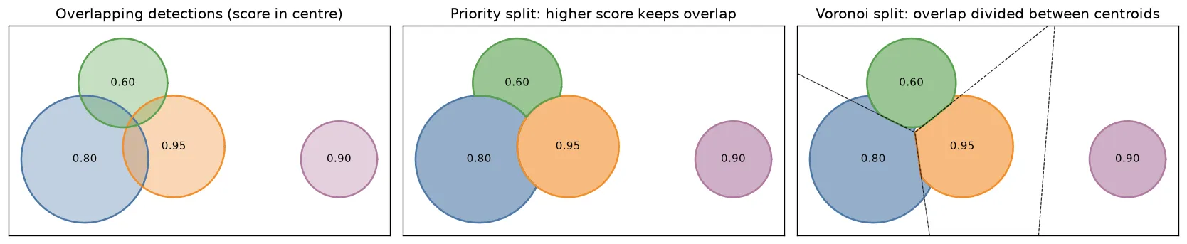
There’s no single right answer. The common approaches are:

Approach	What happens to the overlap	Good when	Cost
Suppress duplicates (NMS on IoU)	the weaker polygon is removed entirely	both polygons describe the same object	loses a real object if the threshold is too low
Priority	goes whole to the more trusted polygon	there is a clear ranking (score, class, source)	the weaker polygon gets a bite taken out
Geometric split (bisector / Voronoi)	divided between the polygons	neither polygon deserves it more	ignores which prediction was better
Merge	polygons are united into one	the parts are pieces of one object	wrong when they are two objects

The second and third need a bit of code.

By priority. Give the whole overlap to the polygon you trust more, usually the one with the higher model score. Each polygon subtracts the union of its stronger neighbours:

def neighbours(k, i, j):
    return np.concatenate([j[i == k], i[j == k]])

def split_by_priority(polys, scores, i, j):
    rank = np.argsort(np.argsort(-scores, kind="stable"))   # 0 = most confident; ties by order
    out = polys.copy()
    for k in range(len(polys)):
        nb = neighbours(k, i, j)
        stronger = nb[rank[nb] < rank[k]]
        if stronger.size:
            out[k] = polys[k].difference(shapely.union_all(polys[stronger]))
    return out

It’s easy to flip the comparison by accident. If you subtract neighbours with a score lower or equal to your own, you get the opposite of what you want: the most confident polygon gets cut by every weaker one, and two polygons with equal scores cut each other, so the overlap belongs to nobody. A strict ranking with a tie-breaker avoids both problems.

Fairly, with Voronoi cells. When neither polygon deserves the overlap more, split it. For two polygons, the natural cut is the perpendicular bisector between their centroids: every point of the overlap goes to the nearer centre. For many polygons, that rule is exactly the Voronoi diagram of the centroids. Each polygon keeps the part nobody else claims, plus the bit of its overlap that falls in its own cell:

def split_by_voronoi(polys, i, j):
    seeds = shapely.multipoints(shapely.centroid(polys))
    box = shapely.union_all(polys).envelope
    cells = shapely.voronoi_polygons(seeds, extend_to=box, ordered=True)  # cell k <-> seed k
    out = polys.copy()
    for k in range(len(polys)):
        nb = neighbours(k, i, j)
        if nb.size:
            own = polys[k].difference(shapely.union_all(polys[nb]))     # uncontested
            out[k] = own.union(polys[k].intersection(cells.geoms[k]))   # + its share
    return out

ordered=True (GEOS 3.12 or newer) keeps cell $k$ lined up with seed $k$. Both methods give polygons that don’t overlap anymore. The Voronoi split has two limits. The bisector ignores size, so a big object loses as much to a small neighbour as the other way round (a weighted, or power, diagram fixes that). And in a cluster of three or more, a sliver of overlap can land in the cell of a polygon that doesn’t contain it, and then it just gets dropped. That’s a fraction of a percent in the example above, but check the total area if it matters.

Key takeaways

• Checking all pairs for overlap is $O(n^2)$. An STRtree makes it about $O(n \log n)$ by filtering on bounding boxes first.
• In Shapely 2, STRtree(geoms).query(geoms, predicate="intersects") returns all index pairs. Drop i >= j.
• query returns integer positions, not geometries, and without a predicate it’s only a box test.
• Group pairs into connected components and handle each cluster on its own.
• Overlaps can be suppressed, given to the stronger polygon, split by Voronoi cells or merged. The right choice depends on whether the polygons are really the same object.

Resources

• Shapely documentation: STRtree, voronoi_polygons, union_all, and the Shapely 2.0 migration guide (the change from geometries to indices in STRtree.query).
• GeoPandas documentation: SpatialIndex.query and sjoin.
• SciPy documentation: csgraph.connected_components.
• Leutenegger, S. T., Lopez, M. A. & Edgington, J. (1997). STR: A simple and efficient algorithm for R-tree packing. Proceedings of the 13th International Conference on Data Engineering (ICDE), 497–506.
• Guttman, A. (1984). R-trees: A dynamic index structure for spatial searching. Proceedings of ACM SIGMOD, 47–57.
• Aurenhammer, F. (1991). Voronoi diagrams: a survey of a fundamental geometric data structure. ACM Computing Surveys, 23(3), 345–405.