The discrete Fourier transform of images: magnitude, phase and shifts

The Fourier transform describes an image by how much of each spatial frequency it has: slow changes like smooth shading, and fast changes like edges and texture. It’s also the natural way to think about linear, shift-invariant filters such as blurring. I worked through this while reading Chapter 16 of Foundations of Computer Vision (Torralba, Isola and Freeman). These are the parts that made it click for me.

Images as sums of waves

In 1D, a signal with $N$ samples can be written as a sum of $N$ complex sinusoids. In 2D, the building blocks are 2D waves, like ripples running across the image. A real 2D wave on an $N \times M$ grid looks like

$$s[n, m] = A\cos\left(2\pi\left(\frac{u\,n}{N} + \frac{v\,m}{M}\right) + \theta\right),$$

where $n, m$ are pixel coordinates, $u$ and $v$ are how many cycles fit across the image in each direction, $A$ is the amplitude and $\theta$ is the phase. The pair $(u, v)$ sets both how fast the wave wiggles and which way its stripes run.

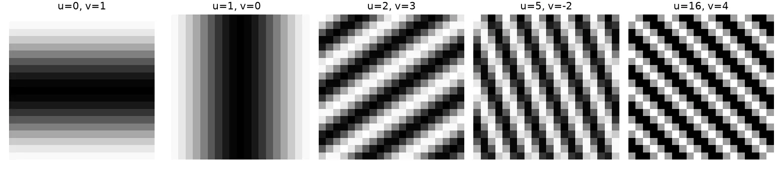
The Fourier transform uses complex exponentials instead, $e^{\,j2\pi(un/N + vm/M)}$. Their real part is a cosine and their imaginary part is a sine, so one complex number per frequency stores both the amplitude and the phase. Look at the last panel, $(u, v) = (16, 4)$ on a 20-pixel grid: it looks exactly like $(-4, 4)$, because frequencies above $N/2$ wrap around. That’s aliasing, which I wrote about in Sampling and aliasing.

The 2D DFT

The discrete Fourier transform of an image $\ell[n, m]$ is

$$\mathcal{L}[u, v] = \sum_{n=0}^{N-1}\sum_{m=0}^{M-1} \ell[n, m]\, e^{-j2\pi\left(\frac{un}{N} + \frac{vm}{M}\right)},$$

and the inverse is

$$\ell[n, m] = \frac{1}{NM}\sum_{u=0}^{N-1}\sum_{v=0}^{M-1} \mathcal{L}[u, v]\, e^{\,j2\pi\left(\frac{un}{N} + \frac{vm}{M}\right)}.$$

The inverse is the easier one to read: the image is a weighted sum of complex exponentials, and $\mathcal{L}[u, v]$ is the weight of each one.

In 1D the DFT is just a matrix product, $\mathcal{L} = F\ell$, with $F[u, n] = e^{-j2\pi un/N}$. Every entry has size 1; only the angle changes. Row $u$ turns by $2\pi u/N$ per step, so row 0 is constant, low rows turn slowly, and rows near $N/2$ turn fastest.

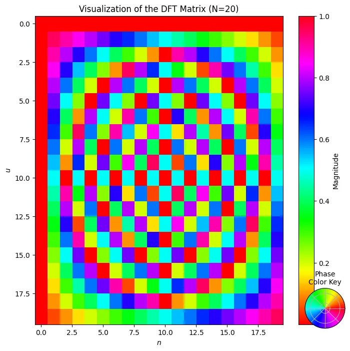
import numpy as np

N = 20
n = np.arange(N)
F = np.exp(-2j * np.pi * np.outer(n, n) / N)   # F[u, n]

x = np.random.rand(N)
print(np.allclose(F @ x, np.fft.fft(x)))       # True: the FFT computes F @ x

The FFT gives the same answer, just faster: $O(N\log N)$ time instead of $O(N^2)$.

Magnitude and phase

Each DFT value is a complex number, so we can write it in polar form:

$$\mathcal{L}[u, v] = A[u, v]\, e^{\,j\theta[u, v]}, \qquad A = |\mathcal{L}|, \quad \theta = \angle\mathcal{L}.$$

In the inverse transform, $A$ says how strongly each sinusoid shows up and $\theta$ says where it’s positioned. To plot the spectrum, we move the zero frequency to the centre with np.fft.fftshift and show $\log(1 + A)$, because the low frequencies are many orders of magnitude stronger than the high ones.

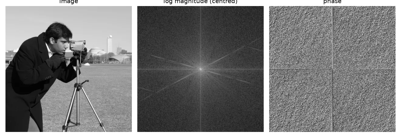
The magnitude looks structured. It’s bright in the centre and fades with frequency, and strong straight edges in the image show up as lines through the centre, at right angles to the edges. The phase just looks like noise. Surprisingly, though, the phase is the more important of the two for what we see.

Shifting the image only changes the phase

Shift the image by $(n_0, m_0)$ pixels (circularly, because the DFT treats the image as if it repeats forever). Then

$$\ell[n - n_0, m - m_0] \;\longleftrightarrow\; \mathcal{L}[u, v]\, e^{-j2\pi\left(\frac{un_0}{N} + \frac{vm_0}{M}\right)}.$$

The extra factor has size 1, so the magnitude spectrum doesn’t change at all. The phase just gets an extra term that grows linearly with frequency. This is the 2D version of the linear phase shift I’d seen with seismic wavelets (see Seismic wavelets: amplitude and phase spectra).

img = np.zeros((5, 5)); img[1:4, 1:4] = 1; img[2, 2] = 0   # small square ring
L = np.fft.fft2(img)
N, M = img.shape
u = np.fft.fftfreq(N).reshape(-1, 1) * N    # integer frequencies in FFT order
v = np.fft.fftfreq(M).reshape(1, -1) * M

n0, m0 = 1, 2
shifted = np.fft.ifft2(L * np.exp(-2j*np.pi*(u*n0/N + v*m0/M))).real
print(np.allclose(shifted, np.roll(img, (n0, m0), axis=(0, 1))))  # True
print(np.allclose(np.abs(np.fft.fft2(shifted)), np.abs(L)))       # True

A mistake I made at first: I multiplied the centred spectrum (after fftshift) by an exponential built from fftfreq, which is in uncentred order. The frequencies don’t line up, and you don’t get a clean shift. Either work with the uncentred spectrum, like above, or shift both.

Phase holds the structure

A classic experiment: take two images, swap their phase spectra, and invert.

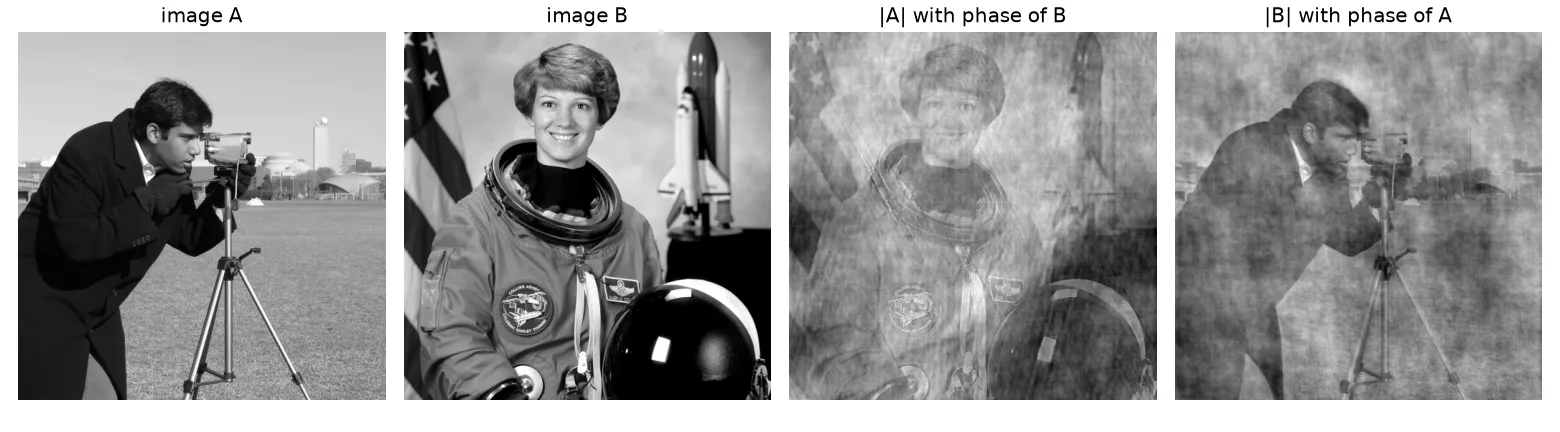
Each result looks like the image its phase came from. The way I think about it: edges show up where lots of sinusoids line up, and the phase decides where they line up. So the phase decides where edges and outlines are. The magnitude mostly sets the overall contrast and the balance between coarse and fine detail. Short version: where things are goes into the phase, how strong they are goes into the magnitude.

That doesn’t make the magnitude useless. It’s a good description of strongly repeating patterns and textures, and it doesn’t change when the image moves. But for natural images, most of the structure you’d recognise lives in the phase.

Why Fourier fits linear filters so well

Complex exponentials are eigenfunctions of every linear shift-invariant system. In plain words: feed one in, and what comes out is the same complex exponential, just multiplied by a complex number (so a new amplitude and a new phase). That means a filter is completely described by one complex number per frequency, its frequency response $H[u, v]$, and filtering becomes simple multiplication:

$$\ell * h \;\longleftrightarrow\; \mathcal{L}[u, v]\, H[u, v].$$

A low-pass filter keeps the centre of the spectrum and throws away the rest, which blurs the image. More on this in Linear filters and Gaussian blur.

How sensitive are we to each frequency?

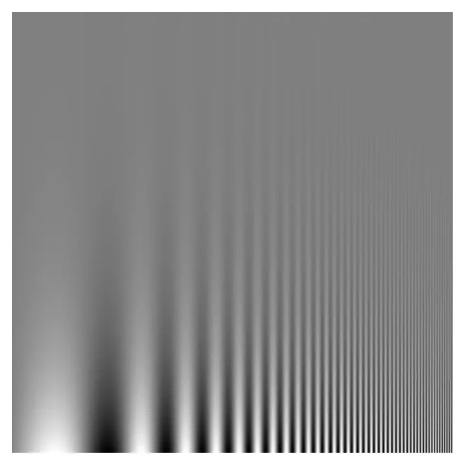
The Campbell–Robson chart shows a sinusoid whose frequency goes up from left to right and whose contrast goes down from bottom to top. The line where the stripes seem to fade into grey traces your own contrast sensitivity function: we can see middle frequencies at lower contrast than very low or very high ones.

Key takeaways

• The 2D DFT writes an image as a weighted sum of complex sinusoids. Each weight has a magnitude and a phase.
• The 1D DFT is just a matrix product with entries of size 1. The FFT is a fast way to compute it.
• Shifting an image only changes the phase, by a term that’s linear in frequency.
• Phase holds most of the visible structure (edges and where they are). Magnitude holds contrast and texture energy.
• Complex exponentials pass through linear shift-invariant filters unchanged except for a scale factor, so filtering is multiplication in the frequency domain.

Resources

• Antonio Torralba, Phillip Isola and William T. Freeman, Foundations of Computer Vision, MIT Press, 2024, Chapter 16 “Fourier Analysis” (DFT, shift property in 16.7, magnitude and phase as an image representation in 16.9, Campbell–Robson chart in 16.10): https://visionbook.mit.edu/image_processing_fourier.html
• NumPy numpy.fft documentation (FFT conventions, fftfreq, fftshift): https://numpy.org/doc/stable/reference/routines.fft.html
• A. V. Oppenheim and J. S. Lim, “The importance of phase in signals”, Proceedings of the IEEE 69(5), 1981 (the classic magnitude/phase swap experiment).
• Test images in the figures: camera and astronaut from scikit-image’s skimage.data: https://scikit-image.org/docs/stable/api/skimage.data.html