Sinkhorn–Knopp: balancing a matrix, and why it solves optimal transport

A lot of problems come down to matching one set of things to another: detections to ground-truth boxes, keypoints in one image to keypoints in another, images to cluster prototypes. The exact answer is a hard one-to-one assignment, and you can’t take gradients through that. The Sinkhorn–Knopp algorithm gives a soft answer instead. What I like about it is how small it is: a loop of two lines (normalise the rows, then the columns). And the same loop, run on the right matrix, solves an entropy-regularised optimal transport problem.

Doubly stochastic matrices

A square matrix with non-negative entries is doubly stochastic when every row and every column sums to 1. The way I read entry $D_{ij}$ is “the fraction of source $i$ that goes to target $j$”. Rows summing to 1 means each source sends out all of its mass. Columns summing to 1 means each target gets exactly one unit.

A permutation matrix is the extreme case: each source goes completely to one target. Birkhoff’s theorem says every doubly stochastic matrix is a weighted average (a convex combination) of permutation matrices. So you can think of a doubly stochastic matrix as a “soft permutation”, and the set of all of them is the natural smooth version of the assignment problem.

The algorithm

Sinkhorn and Knopp (1967) proved a simple fact. Take a square matrix $A$ whose entries are all strictly positive. Divide every row by its sum, then every column by its sum, and keep repeating. The matrix converges to a doubly stochastic matrix $D$, and that $D$ is unique.

import numpy as np

def sinkhorn_knopp(A, tol=1e-9, max_iter=10_000):
    A = np.array(A, dtype=float)
    for it in range(max_iter):
        A /= A.sum(axis=1, keepdims=True)   # rows sum to 1
        A /= A.sum(axis=0, keepdims=True)   # columns sum to 1
        # columns are exact after the last step, so only rows need checking
        if np.abs(A.sum(axis=1) - 1).max() < tol:
            return A, it + 1
    return A, max_iter

D, n_iter = sinkhorn_knopp(np.arange(1, 10).reshape(3, 3))
print(D.round(4), n_iter)
# [[0.2424 0.3489 0.4087]
#  [0.3646 0.328  0.3074]
#  [0.3929 0.3231 0.2839]]  6

Six rounds are enough here. Each step fixes one set of sums and slightly breaks the other, but for a positive matrix the error shrinks geometrically, so it settles quickly.

The result always looks like $D = \operatorname{diag}(r)\, A\, \operatorname{diag}(c)$ for two positive vectors $r$ and $c$. This took me a moment to see: every row division multiplies a row by a number, and every column division multiplies a column by a number, so multiplying all those numbers together gives $r$ and $c$. So the algorithm is really just searching for two scaling vectors. You only need to keep those, not the whole matrix at every step. That’s the form used below.

When there are zeros. If $A$ has zeros, the result may not exist, or it may take a long time to get there. The matrix $\begin{pmatrix}1&1\\0&1\end{pmatrix}$ can only be balanced into the identity, which means the top-right entry has to go to zero. It does, but only like $1/(2k)$ after $k$ rounds (0.0050 after 100 rounds, 0.0005 after 1000). The exact condition for a perfect balance is that $A$ has total support: every non-zero entry lies on some permutation that avoids the zeros.

From balancing to optimal transport

Optimal transport asks this: you have a source distribution $a$ (a histogram with $n$ bins), a target distribution $b$ (with $m$ bins), and a cost $C_{ij}$ for moving one unit of mass from bin $i$ to bin $j$. What’s the cheapest plan $P$ that moves all of $a$ onto $b$?

$$\min_{P \ge 0} \; \sum_{ij} P_{ij} C_{ij} \quad \text{subject to} \quad P\mathbf{1} = a, \;\; P^\top \mathbf{1} = b .$$

The constraints just say the row sums of $P$ are $a$ and the column sums are $b$. With $a = b = \mathbf{1}/n$ and $n$ items on each side, this is the assignment problem: there’s always an optimal plan that is a permutation matrix divided by $n$. When $C_{ij}$ is a distance $d(x_i, y_j)$ raised to a power $p \ge 1$, the optimal cost is the Wasserstein distance $W_p^p$ (for $p = 1$, the earth mover’s distance). Solving it exactly is a linear program, roughly $O(n^3)$, and the solution jumps when $C$ changes, so you can’t backpropagate through it cleanly.

Cuturi (2013) added an entropy term that rewards spread-out plans:

$$\min_{P \ge 0} \; \sum_{ij} P_{ij} C_{ij} \;-\; \varepsilon\, H(P), \qquad H(P) = -\sum_{ij} P_{ij} (\log P_{ij} - 1).$$

Here $\varepsilon > 0$ controls how much blur we’re willing to accept. If you set the derivative to zero, the optimal plan turns out to have the form

$$P = \operatorname{diag}(u)\, K\, \operatorname{diag}(v), \qquad K_{ij} = e^{-C_{ij}/\varepsilon}.$$

And that’s exactly the Sinkhorn–Knopp form. The “Gibbs kernel” $K$ is positive, and all we need are the scalings $u$ and $v$ that give the right row sums $a$ and column sums $b$. Switching back and forth between the two conditions gives the Sinkhorn iterations:

def sinkhorn(a, b, C, eps, n_iter=1000):
    K = np.exp(-C / eps)          # cheap moves get large weights
    v = np.ones_like(b)
    for _ in range(n_iter):
        u = a / (K @ v)           # match row sums to a
        v = b / (K.T @ u)         # match column sums to b
    return u[:, None] * K * v[None, :]

Each iteration is just two matrix–vector products, so it’s fast, easy to batch on a GPU, and differentiable all the way through. The plain Sinkhorn–Knopp loop from the first section is the special case $K = A$, $a = b = \mathbf{1}$.

What ε does

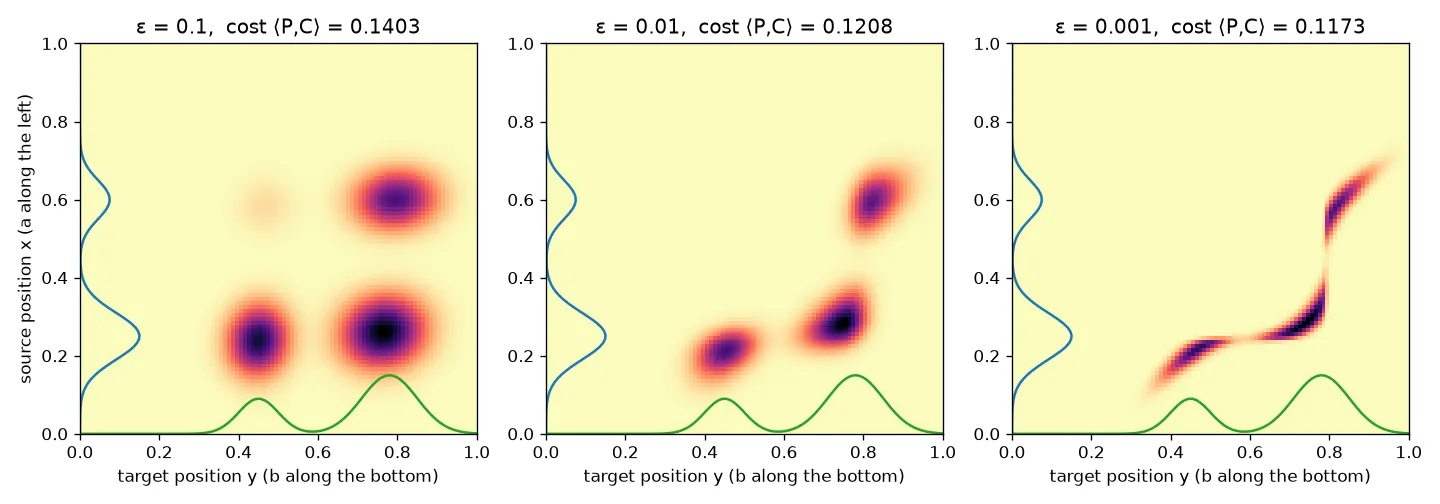
• Large ε: the entropy term wins. The plan tends to $a b^\top$, which sends every source everywhere, and it converges in a few iterations.
• Small ε: the plan gets close to the exact optimal plan. On a random $5 \times 5$ cost matrix, the arg-max of each row of $P$ matched the Hungarian algorithm’s assignment for $\varepsilon = 0.1$ and below, and the cost at $\varepsilon = 0.01$ was within 0.1% of the exact optimum.

Small ε comes at two costs. Convergence gets much slower, so you need many more iterations. And $e^{-C/\varepsilon}$ underflows to zero: with random costs in $[0, 1]$ and $\varepsilon = 10^{-4}$, the plain loop above returns nan. The usual fix is to run the same iteration on logarithms, with dual potentials $f = \varepsilon \log u$ and $g = \varepsilon \log v$ and a numerically stable log-sum-exp:

from scipy.special import logsumexp

def sinkhorn_log(a, b, C, eps, n_iter=1000):
    f, g = np.zeros_like(a), np.zeros_like(b)
    for _ in range(n_iter):
        f = eps * (np.log(a) - logsumexp((g[None, :] - C) / eps, axis=1))
        g = eps * (np.log(b) - logsumexp((f[:, None] - C) / eps, axis=0))
    return np.exp((f[:, None] + g[None, :] - C) / eps)

Libraries like POT and GeomLoss implement this log-domain version, plus tricks like slowly lowering ε.

Where it shows up in machine learning

• Feature matching. SuperGlue matches keypoints between two images by running Sinkhorn on a learned score matrix, with an extra “dustbin” row and column for points that don’t have a match.
• Self-supervised learning. SwAV, and later DINOv2, use a few Sinkhorn–Knopp steps to spread a batch evenly over the prototypes. That stops all images from collapsing onto one cluster (see DINOv2).
• Losses between distributions. Sinkhorn divergences compare point clouds, histograms or generated samples and stay differentiable.
• Older uses. The same row-and-column scaling is called iterative proportional fitting (adjusting a survey table to known totals) and the RAS method for balancing economic input–output tables.

Key takeaways

• If you keep normalising the rows and columns of a positive square matrix, it converges to a unique doubly stochastic matrix $\operatorname{diag}(r) A \operatorname{diag}(c)$.
• A doubly stochastic matrix is a soft permutation: a mix of hard assignments (Birkhoff).
• Entropy-regularised optimal transport has a solution of the same form with $K = e^{-C/\varepsilon}$, so the Sinkhorn loop solves it using only matrix–vector products.
• ε trades accuracy for speed and smoothness. For small ε, work in the log domain to avoid underflow.
• Zeros in the matrix can make balancing slow or impossible, so check for total support.

Resources

• R. Sinkhorn and P. Knopp, “Concerning nonnegative matrices and doubly stochastic matrices”, Pacific Journal of Mathematics 21(2), 1967.
• M. Cuturi, “Sinkhorn Distances: Lightspeed Computation of Optimal Transport”, NeurIPS 2013. https://arxiv.org/abs/1306.0895
• G. Peyré and M. Cuturi, Computational Optimal Transport, 2019, Chapter 4 (entropic regularisation and Sinkhorn). https://arxiv.org/abs/1803.00567
• P.-E. Sarlin et al., “SuperGlue: Learning Feature Matching with Graph Neural Networks”, CVPR 2020. https://arxiv.org/abs/1911.11763
• M. Caron et al., “Unsupervised Learning of Visual Features by Contrasting Cluster Assignments” (SwAV), NeurIPS 2020. https://arxiv.org/abs/2006.09882
• POT: Python Optimal Transport library. https://pythonot.github.io/