DINOv2: learning visual features without labels

Most vision models learn from labels: someone has to say “cat” or draw a box. DINOv2 learns from raw images alone. Its features are good enough that a single linear layer on top can classify, segment or estimate depth. So if you want a good general-purpose image backbone and you don’t have labels, DINOv2 is one of the first things to try. Here I write down how it’s trained and how to use what comes out.

The idea: a student copies a teacher

DINOv2 (“self-DIstillation with NO labels”, version 2) uses two Vision Transformers with the same architecture:

The student is trained with gradient descent.
The teacher gets no gradients. Its weights are an exponential moving average (EMA) of the student’s weights.

Both networks see different random views of the same image, and the student has to predict what the teacher outputs. The teacher is a smoothed, slightly older copy of the student, so it gives a steady target. The way I think about it: there are no labels anywhere, but the game still forces the network to describe an image in a way that doesn’t change when you crop, flip or recolor it.

The EMA update for each teacher weight $\theta_t$ is

\theta_t \leftarrow m\,\theta_t + (1-m)\,\theta_s

where $\theta_s$ is the matching student weight and $m$ is a momentum close to 1. So the teacher moves only a tiny bit towards the student each step (DINOv2 raises $m$ from 0.992 towards 1 with a cosine schedule).

@torch.no_grad()
def update_teacher(student, teacher, m=0.992):
    for p_s, p_t in zip(student.parameters(), teacher.parameters()):
        p_t.mul_(m).add_((1 - m) * p_s)

Views: global and local crops

Each image becomes several crops (multi-crop augmentation):

2 global crops: large crops (more than about a third of the image), resized to 224×224.
Several local crops (typically 8): small crops, resized to 98×98 in DINOv2 (96×96 in the original DINO).

The teacher only sees the global crops, while the student sees all of them. So the student has to guess what the whole scene looks like from a small piece. That pushes it to link local details to the global picture.

import torchvision.transforms as T

norm = T.Normalize([0.485, 0.456, 0.406], [0.229, 0.224, 0.225])
global_tf = T.Compose([T.RandomResizedCrop(224, scale=(0.32, 1.0)),
                       T.RandomHorizontalFlip(), T.ColorJitter(0.4, 0.4, 0.2, 0.1),
                       T.ToTensor(), norm])
local_tf = T.Compose([T.RandomResizedCrop(98, scale=(0.05, 0.32)),
                      T.RandomHorizontalFlip(), T.ColorJitter(0.4, 0.4, 0.2, 0.1),
                      T.ToTensor(), norm])

The backbone: a Vision Transformer with patch size 14

The image is cut into 14×14-pixel patches. A convolution with kernel size and stride both 14 does the cutting and the linear projection in one go. A learnable [CLS] token (an extra token meant to collect a summary of the image) goes in front of the patch tokens, and positional embeddings are added. For a 224×224 input that’s $16 \times 16 = 256$ patch tokens plus one [CLS] token, so 257 tokens.

After the transformer:

the [CLS] token summarizes the whole image (good for classification and retrieval);
the patch tokens describe each local region (good for segmentation and depth).

Three losses

1. DINO loss (image level)

The [CLS] outputs of the student and the teacher go through a projection head that gives scores over $K$ “prototypes” (think of them as learned pseudo-classes, e.g. $K = 65{,}536$ ). Each score vector is turned into a probability distribution with a softmax at temperature $\tau$ :

P(x)^{(k)} = \frac{\exp(g(x)^{(k)}/\tau)}{\sum_{j=1}^{K} \exp(g(x)^{(j)}/\tau)}

Here $g(x)^{(k)}$ is the head’s score for prototype $k$ . The loss is the cross-entropy $-\sum_k P_t^{(k)} \log P_s^{(k)}$ between the teacher’s distribution $P_t$ (from one view) and the student’s distribution $P_s$ (from a different view). The teacher uses a low temperature, which makes its targets sharper. In the original DINO, the teacher outputs are also centered (a running mean is subtracted) so that one prototype can’t win every time. DINOv2 swaps centering for Sinkhorn-Knopp normalization (from SwAV), which evens out how often each prototype gets used.

import torch.nn.functional as F

def dino_loss(student_logits, teacher_logits, center, t_s=0.1, t_t=0.04):
    # student and teacher logits come from DIFFERENT views of the same image
    p_t = F.softmax((teacher_logits - center) / t_t, dim=-1).detach()
    log_p_s = F.log_softmax(student_logits / t_s, dim=-1)
    return -(p_t * log_p_s).sum(dim=-1).mean()

2. iBOT loss (patch level)

Some patches of the student’s global crops are masked: their embeddings are swapped for a learnable mask token (they’re not dropped like in MAE). The teacher sees the same crop with nothing hidden. For every masked spot, the student has to predict the teacher’s patch distribution at that spot, with the same kind of cross-entropy. So basically it’s fill-in-the-blank for images, the visual version of BERT. This is the part that makes the patch features useful for dense tasks like segmentation.

def mask_patches(x, mask_token, ratio=0.5):
    # x: (B, N, D) patch embeddings, mask_token: (1, 1, D) learnable
    B, N, _ = x.shape
    mask = torch.rand(B, N, device=x.device) < ratio      # True = masked
    x = torch.where(mask.unsqueeze(-1), mask_token.expand(B, N, -1), x)
    return x, mask

DINOv2 uses separate (untied) heads for the DINO and iBOT losses. The paper found that this works better at large scale than sharing one head.

3. KoLeo regularizer (keep the features spread out)

A self-supervised model can “cheat” by mapping every image to almost the same vector (this is called collapse). The KoLeo regularizer, based on the Kozachenko-Leonenko entropy estimator, pushes the features in a batch away from each other:

\mathcal{L}_{\text{KoLeo}} = -\frac{1}{n}\sum_{i=1}^{n} \log d_{n,i}, \qquad d_{n,i} = \min_{j \neq i} \lVert x_i - x_j \rVert

Here $x_i$ is the L2-normalized [CLS] feature of image $i$ , $n$ is the batch size and $d_{n,i}$ is the distance to its nearest neighbor in the batch. If two features get close, the log of that small distance is very negative, so the loss goes up.

def koleo(x, eps=1e-8):
    x = F.normalize(x, dim=-1)
    d = torch.cdist(x, x)
    d.fill_diagonal_(float("inf"))          # ignore distance to itself
    return -torch.log(d.min(dim=1).values + eps).mean()

The total loss is $\mathcal{L}_{\text{DINO}} + \mathcal{L}_{\text{iBOT}} + \lambda\,\mathcal{L}_{\text{KoLeo}}$ with a small $\lambda$ (0.1).

What else changed from DINO to DINOv2

Data: LVD-142M, 142 million images picked automatically from a big messy pool. They kept images that look similar to ones in curated datasets and removed near-duplicates.
Scale: the biggest model is ViT-g (about 1.1B parameters, with SwiGLU feed-forward layers). The smaller models (ViT-S/B/L) are distilled from it, not trained from scratch.
High-resolution finish: for a short stretch at the end of training, the resolution goes up to 518×518. More pixels means more patches, so the model picks up finer detail.

Using a pretrained DINOv2

With Hugging Face Transformers, getting features out only takes a few lines. I tried it on the COCO image of two cats on a sofa.

from transformers import AutoImageProcessor, AutoModel
import torch

processor = AutoImageProcessor.from_pretrained("facebook/dinov2-small")
model = AutoModel.from_pretrained("facebook/dinov2-small")

inputs = processor(images=image, return_tensors="pt")   # resize 256, center-crop 224
with torch.no_grad():
    out = model(**inputs)

tokens = out.last_hidden_state          # (1, 257, 384)
cls, patches = tokens[:, 0], tokens[:, 1:]
feature_map = patches.transpose(1, 2).unflatten(2, (16, 16))   # (1, 384, 16, 16)

The last line turns the 256 patch tokens back into a 16×16 grid with 384 channels. Now it looks just like a CNN feature map. You can put a segmentation head on it, or take tokens from several middle blocks to build a feature pyramid for a detector like Mask R-CNN.

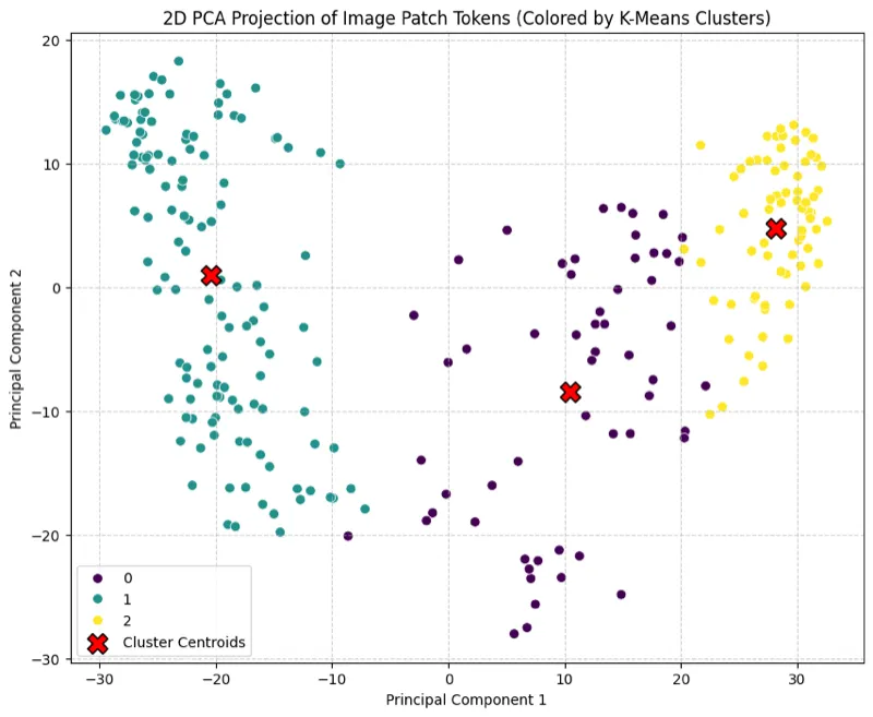
A quick way to see how good the features are: run k-means (3 clusters) on the 256 patch vectors and project them with PCA. The patches fall into three clearly separate groups, and I didn’t train anything. If you map the cluster labels back onto the 16×16 grid, you get a rough segmentation for free.

PCA projection of the 256 DINOv2 patch tokens of the two-cats image, colored by three k-means clusters that form clearly separated groups

Two things that caught me out while trying this:

The processor center-crops the image. If you lay a 16×16 attention or similarity map over the full original image, it won’t line up. Lay it over the cropped image instead, or turn cropping off.
Attention maps from the first layer mostly show low-level patterns. The object-shaped attention maps DINO is famous for show up in the last layer (outputs.attentions[-1]).

Key takeaways

DINOv2 learns by making a student match an EMA teacher across different crops of the same image. No labels needed.
The DINO loss works on the [CLS] token (the whole-image meaning), the iBOT loss works on masked patch tokens (local detail), and KoLeo keeps the features spread out.
Teacher centering or Sinkhorn-Knopp normalization, sharpening and the EMA update together stop the model from collapsing.
The patch tokens can be reshaped into a 2D feature map and used straight away for dense tasks.
Lots of curated data and a short high-resolution phase at the end are a big part of why DINOv2 works so well.

Resources

Oquab et al., “DINOv2: Learning Robust Visual Features without Supervision”, TMLR 2024. arXiv:2304.07193
Caron et al., “Emerging Properties in Self-Supervised Vision Transformers” (DINO), ICCV 2021. arXiv:2104.14294
Zhou et al., “iBOT: Image BERT Pre-Training with Online Tokenizer”, ICLR 2022. arXiv:2111.07832
Sablayrolles et al., “Spreading vectors for similarity search” (KoLeo), ICLR 2019. arXiv:1806.03198
Official code: facebookresearch/dinov2
Hugging Face docs: DINOv2 and the model card facebook/dinov2-small