Backprop by hand through an MLP language model
Writing the backward pass of a character-level MLP by hand, one tensor at a time, including the short formula for the softmax cross-entropy gradient and the scatter-add for the embedding table, and checking every step against PyTorch autograd.
loss.backward() is one line, and it hides a lot. When training goes wrong (dead units, exploding gradients, a shape bug that doesn’t throw an error), it helps to know what actually flows backwards through each line of the forward pass. So for this exercise I threw out autograd. I wrote the backward pass for the MLP language model by hand, one tensor at a time, and checked each gradient against PyTorch. The chain rule for single numbers is in my micrograd note. This one is all about tensors, shapes and broadcasting.
The forward pass, cut into small steps
The model turns 3 characters into 10-dimensional vectors, then runs a linear layer, batch normalization and tanh, then an output layer. To make the backward pass doable, I wrote the cross-entropy loss out in tiny steps, so every in-between result has a name.
emb = C[Xb]                                  # (32, 3, 10)
embcat = emb.view(emb.shape[0], -1)          # (32, 30)
hprebn = embcat @ W1 + b1                    # (32, 64)
# ... batch norm produces hpreact ...
h = torch.tanh(hpreact)                      # (32, 64)
logits = h @ W2 + b2                         # (32, 27)
logit_maxes = logits.max(1, keepdim=True).values
norm_logits = logits - logit_maxes           # for numerical stability
counts = norm_logits.exp()
counts_sum = counts.sum(1, keepdim=True)
counts_sum_inv = counts_sum ** -1
probs = counts * counts_sum_inv
logprobs = probs.log()
loss = -logprobs[range(n), Yb].mean()
Each in-between tensor gets retain_grad(), so I can compare my hand-computed gradient dX with PyTorch’s X.grad.
Two rules that sort out most of the shapes
Two simple rules sort out almost all of the shapes.
1. A gradient has the same shape as the thing it belongs to. dW2 has to be (64, 27) because W2 is. That alone often tells you where a transpose goes.
2. Broadcasting and summing are mirror images. This was the most useful thing I took from the whole exercise.
- If a tensor was broadcast (copied) in the forward pass, sum its gradient over the copied dimension in the backward pass. Example:
b2of shape (27,) is added to every row of the (32, 27) logits, sodb2 = dlogits.sum(0). - If a tensor was summed in the forward pass, broadcast the gradient back. Example:
counts_sum = counts.sum(1, keepdim=True), so every element in a row ofcountsgets the gradient of that row’s sum.
And if a variable is used in two places, it collects gradient from both, and you add them up. counts feeds both probs and counts_sum, so dcounts has two parts.
Walking backwards
Below, n is the batch size (32). The loss only averages at the target positions. So dlogprobs is at those 32 entries and 0 everywhere else.
dlogprobs = torch.zeros_like(logprobs)
dlogprobs[range(n), Yb] = -1.0 / n
dprobs = (1.0 / probs) * dlogprobs                       # d log(x) = 1/x
dcounts_sum_inv = (counts * dprobs).sum(1, keepdim=True) # was broadcast
dcounts = counts_sum_inv * dprobs
dcounts_sum = -counts_sum**-2 * dcounts_sum_inv
dcounts += torch.ones_like(counts) * dcounts_sum          # second use
dnorm_logits = counts * dcounts                          # d exp(x) = exp(x)
dlogits = dnorm_logits.clone()
dlogit_maxes = (-dnorm_logits).sum(1, keepdim=True)
dlogits += F.one_hot(logits.max(1).indices, 27) * dlogit_maxes
dlogit_maxes came out as basically zero. It makes sense once you think about it. Subtracting the same number from every logit in a row doesn’t change the softmax, so the loss can’t depend on it. Subtracting the max is only there to stop exp from overflowing.
For a linear layer the rules are
You don’t need to memorize these. Just write the matrix product whose shapes give the shape you need.
dh = dlogits @ W2.T          # (32,27) @ (27,64) -> (32,64)
dW2 = h.T @ dlogits          # (64,32) @ (32,27) -> (64,27)
db2 = dlogits.sum(0)
dhpreact = (1.0 - h**2) * dh # tanh'(x) = 1 - tanh(x)^2
The gradient of cross-entropy in one line
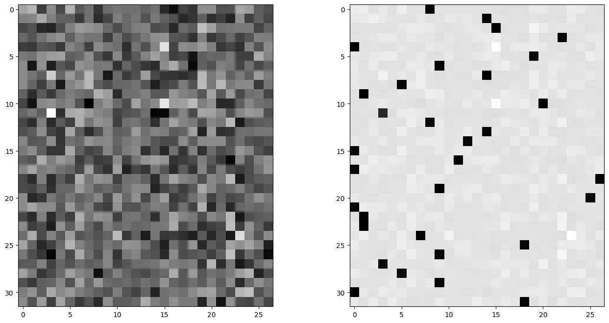
After all that work, the surprise: all eight steps from logits to loss boil down to a short formula. For one example with logits , softmax probabilities and target , the loss is and
Averaging over a batch of examples just divides by :
dlogits = F.softmax(logits, 1)
dlogits[range(n), Yb] -= 1
dlogits /= n
This matched PyTorch to about . I also like how easy it is to read. Every wrong class gets pushed down in proportion to the probability the model gave it. The correct class gets pulled up by . Each row of dlogits adds up to zero, so the pushing and the pulling balance out.
Through batch norm, and into the embedding table
Batch normalization was the trickiest part. It ties all the examples in a batch together through the mean and variance, so its backward pass has several paths. Doing it step by step and then simplifying on paper gives one expression. Here is the normalized pre-activations, the gain, , and the variance is the unbiased one (divide by ):
The sums go over the batch, separately for each of the 64 features. I’m just writing it down here; the layer itself is explained in the batch normalization note.
The last step is the embedding lookup emb = C[Xb]. Each row of C got copied into emb once for every time its character showed up in the batch. So the gradient of a row of C is the sum of the gradients at all the positions that used it. That’s called a scatter-add:
dembcat = dhprebn @ W1.T                       # back through the first linear layer
demb = dembcat.view(emb.shape)                 # undo the flatten
dC = torch.zeros_like(C)
dC.index_add_(0, Xb.view(-1), demb.view(-1, C.shape[1]))
My first version used two nested Python loops over batch and position. Same result, but index_add_ does it in one fast call.
Training with only my own gradients
The real test: with every gradient in place, I removed loss.backward(), wrapped the loop in torch.no_grad(), and trained the network for 200,000 steps using only my hand-written backward pass. The loss went from 3.77 to around 1.9-2.0 on the minibatches, the same as with autograd. That was a satisfying moment. A final check of all parameter gradients against PyTorch showed differences below . Those tiny differences come from floating-point rounding when the math is done in a different order, not from mistakes.
Key takeaways
- A tensor’s gradient always has the same shape as the tensor. Matching shapes tells you where transposes and sums go.
- Broadcast in the forward pass means sum in the backward pass, and sum in the forward pass means broadcast in the backward pass.
- The gradient of softmax cross-entropy with respect to the logits is . It’s cheap, stable and easy to understand.
- Subtracting the max logit has zero gradient. It’s only there to avoid overflow.
- The gradient of an embedding table is a scatter-add: each row adds up the gradients from every position that used it.
Resources
- Andrej Karpathy, “Building makemore Part 4: Becoming a Backprop Ninja”, Neural Networks: Zero to Hero (video): https://www.youtube.com/watch?v=q8SA3rM6ckI. The exercise structure and the step-by-step forward pass come from this lecture.
- Andrej Karpathy, “Yes you should understand backprop” (blog post): https://karpathy.medium.com/yes-you-should-understand-backprop-e2f06eab496b
- Sergey Ioffe and Christian Szegedy, “Batch Normalization”, 2015: https://arxiv.org/abs/1502.03167
- PyTorch documentation,
Tensor.index_add_: https://pytorch.org/docs/stable/generated/torch.Tensor.index_add_.html