Regression error analysis beyond RMSE: what each metric hides and how to look past it
What bias, MAE, RMSE, MAPE and R² each measure and hide, and how residual plots and per-bin and per-group errors show problems that one score can't.
I used to judge a regression model by one number, usually RMSE. Then it hit me that this number is an average over every prediction, so it hides where the model fails. A model can have a nice RMSE and still be badly biased for large values, or for one group of users, or have errors that grow as the target gets bigger. Error analysis is just the habit of breaking the error apart until you know who gets the bad predictions and why.
The usual metrics, and what each one hides
I’ll write the error of prediction as , where is the prediction and the true value, for test samples.
| Metric | Formula | What it rewards | What it hides |
|---|---|---|---|
| Bias (mean error) | Systematic over- or under-prediction | Large errors that cancel out | |
| MAE | Typical error size; not thrown off much by outliers | How big the worst errors are | |
| RMSE | Penalizes large errors heavily | Driven by a few large cases; scale-dependent | |
| MAPE | Relative error, unit-free | Explodes near ; dominated by small targets | |
| Error relative to predicting the mean | Depends on how spread out the test set is |
A few of these surprised me, so here’s more on them.
MAE versus RMSE. The constant that minimizes MAE is the median, while the one that minimizes squared error is the mean (Gneiting 2011). So the two metrics are actually asking for different predictions. RMSE is always at least as big as MAE. If RMSE/MAE is well above about 1.25 (the value you get for normally distributed errors), that hints at heavy tails: a small number of big misses.
MAPE is lopsided. If the truth is 10, predicting 0 costs 100%, but predicting 30 costs 200%, and over-predicting has no upper limit. So models tuned for MAPE lean towards predicting too low. Small true values also get huge weight. Hyndman and Koehler (2006) go through these problems and suggest scaled alternatives.
isn’t an error. Its denominator is the variance of the test targets. So the same model, with exactly the same errors, gets a higher on a test set that covers a wider range. Use it to compare models on the same data, not to compare datasets.
Bias can cancel out. A mean error near zero only says the overs and unders balance over the whole test set. It says nothing about any subset.
A synthetic example
To see this for real, I made some fake data. It has multiplicative noise (bigger targets, bigger spread) and five groups, and one of them (E) runs higher than the rest. The model is a plain linear fit that doesn’t know about the groups.
import numpy as np
from sklearn.linear_model import LinearRegression
from sklearn.model_selection import train_test_split

rng = np.random.default_rng(0)
n = 3000
group = rng.choice(list("ABCDE"), n)
x = rng.uniform(1, 10, n)
# Multiplicative noise (spread grows with size) and one group that runs high
y = 4 * x * np.exp(rng.normal(0, 0.25, n)) + np.where(group == "E", 4.0, 0.0)

x_tr, x_te, y_tr, y_te, g_tr, g_te = train_test_split(x, y, group, random_state=0)
model = LinearRegression().fit(x_tr[:, None], y_tr)
y_hat = model.predict(x_te[:, None])
e = y_hat - y_te                                  # error = prediction - truth

def summary(y, y_hat):
    e = y_hat - y
    return {
        "bias": e.mean(),
        "MAE": np.abs(e).mean(),
        "RMSE": np.sqrt((e ** 2).mean()),
        "MAPE %": 100 * np.abs(e / y).mean(),
        "R2": 1 - (e ** 2).sum() / ((y - y.mean()) ** 2).sum(),
    }
print({k: round(float(v), 2) for k, v in summary(y_te, y_hat).items()})
# {'bias': 0.3, 'MAE': 4.77, 'RMSE': 6.58, 'MAPE %': 23.94, 'R2': 0.7}
Bias 0.3, . Looks fine. Now let’s look inside.
Plot the residuals, two ways
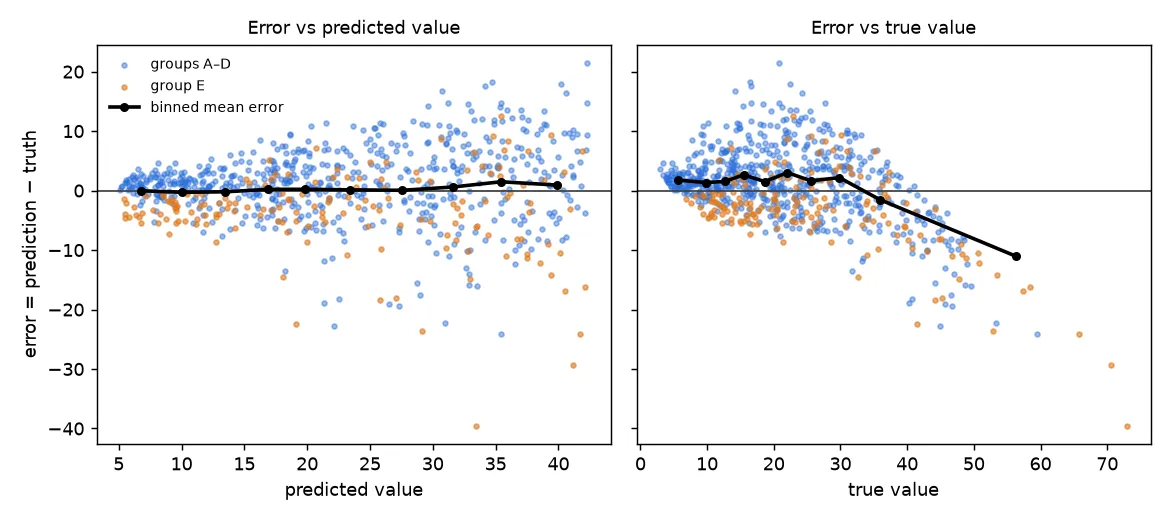
Error against prediction (left). This is the classic residual plot, and two things show up. First, a funnel: the spread grows with the predicted value. The fancy name is heteroscedasticity, which just means the error variance isn’t constant. A single RMSE mixes the small errors at the low end with the big errors at the high end, so it describes neither. Second, the orange points (group E) sit mostly below zero: the model under-predicts that group.
Error against truth (right). Here the binned mean error slopes down: small true values get over-predicted, large ones under-predicted. This is the view users actually feel. Someone whose true value is large gets an estimate that’s too low. But this tripped me up at first: the slope shows up for any imperfect model, even one whose predictions are perfectly calibrated (). When you pick cases with an extreme true value, you also pick cases where the noise pushed them up, and the model can’t see that noise, so it falls short. That’s regression to the mean. If you “stretch” the predictions to remove the slope, the overall error gets worse.
So both views are useful; they just answer different questions. Binning by prediction asks “when the model says 30, is the truth 30 on average?” (calibration). Binning by truth asks “how wrong is the model for cases that really are large?” (risk at the extremes).
Break the score down
The same summary function, run inside bins and groups, turns one number into a table:
def binned(by, n_bins=5):
    # Metrics within quantile bins of `by` (equal counts per bin)
    edges = np.quantile(by, np.linspace(0, 1, n_bins + 1))
    idx = np.clip(np.digitize(by, edges[1:-1]), 0, n_bins - 1)
    for b in range(n_bins):
        s = summary(y_te[idx == b], y_hat[idx == b])
        print(f"  [{edges[b]:5.1f}, {edges[b+1]:5.1f}]  bias={s['bias']:+5.2f}  "
              f"MAE={s['MAE']:5.2f}  MAPE={s['MAPE %']:5.1f}%")

print("binned by TRUE value");      binned(y_te)
print("binned by PREDICTED value"); binned(y_hat)
for g in "ABCDE":
    m = g_te == g
    print(g, f"bias={summary(y_te[m], y_hat[m])['bias']:+.2f}")
What the output shows:
- By true value: bias goes from about +2 in the lower bins to −6.3 in the top bin. MAE triples from the lowest bin to the highest, while MAPE drops from 32% to 18%. So absolute and relative error tell opposite stories about which end is “worse”.
- By predicted value: bias stays between −0.2 and +1.2. The model is roughly calibrated, so the strong slope above is mostly regression to the mean.
- By group: groups A–D have a bias of about +1.2 to +1.6, and group E has −3.5. The near-zero overall bias was just these cancelling out. The real problem is a missing feature (which group a row is in), and only the per-group view shows it.
What to do about it
- Funnel-shaped errors: try modelling on a log scale or with a relative loss, report relative metrics next to absolute ones, or predict intervals (for example with quantile regression) instead of one number.
- Group bias points to a missing feature, a data-quality problem in one group, or a group that’s under-represented in training. Validate with grouped folds so you see how the model does on groups it hasn’t seen.
- Tail errors: look at the individual worst cases. Big misses are often label errors, unit mix-ups or inputs outside the training range.
- Small subsets are noisy. Show the count next to every per-bin or per-group metric, and bootstrap a confidence interval before acting on a difference.
Key takeaways
- Every summary metric averages something away: bias cancels, RMSE is driven by the tails, MAPE by small targets, and by how spread out the test set is.
- Plot errors against the prediction (calibration, heteroscedasticity) and against the truth (risk at the extremes), and remember that the second one always slopes.
- Break metrics down by target range and by group. A near-zero overall bias can hide big biases in opposite directions.
- Pick the metric that matches the decision the prediction is for, and report its spread, not just its mean.
Resources
- Rob J. Hyndman, Anne B. Koehler, “Another look at measures of forecast accuracy”, International Journal of Forecasting 22(4) (2006): https://doi.org/10.1016/j.ijforecast.2006.03.001
- Tilmann Gneiting, “Making and Evaluating Point Forecasts”, Journal of the American Statistical Association 106 (2011): https://doi.org/10.1198/jasa.2011.r10138
- Rob J. Hyndman, George Athanasopoulos, Forecasting: Principles and Practice, 3rd ed., Section 5.8: https://otexts.com/fpp3/accuracy.html
- Gareth James, Daniela Witten, Trevor Hastie, Robert Tibshirani, An Introduction to Statistical Learning, Section 3.3.3 (residual plots, non-constant variance): https://www.statlearning.com/
- Cort J. Willmott, Kenji Matsuura, “Advantages of the mean absolute error (MAE) over the root mean square error (RMSE)”, Climate Research 30 (2005): https://doi.org/10.3354/cr030079
- Tianfeng Chai, Roland R. Draxler, “Root mean square error (RMSE) or mean absolute error (MAE)?”, Geoscientific Model Development 7 (2014): https://doi.org/10.5194/gmd-7-1247-2014
- Francis Galton, “Regression towards mediocrity in hereditary stature”, Journal of the Anthropological Institute 15 (1886), the origin of regression to the mean: https://doi.org/10.2307/2841583