Monotonic constraints in gradient-boosted trees: building domain knowledge into the model
What a monotonic constraint is, how boosting libraries enforce it while growing trees, and when it makes a model more accurate and easier to trust.
Often you know the direction of a relationship before you see any data. A bigger house shouldn’t lower the predicted price, all else equal. A higher dose shouldn’t lower the predicted effect in the range you care about. But a flexible model trained on a small, noisy sample doesn’t know that, and it’ll happily learn little dips and bumps that are pure noise. A monotonic constraint tells the model: “along this feature, predictions can only go up” (or only down). It’s one of the cheapest ways to put domain knowledge into a tree ensemble.
What “monotone” means here
Let be the model’s prediction. The model is monotonically increasing in feature if
for every fixed setting of the other features. In plain words: change only , keep everything else the same, and the prediction can never move the wrong way. Decreasing is the same with .
Two details that are easy to miss:
- It’s a ceteris paribus statement (Latin for “other things equal”). It says nothing about the raw correlation between and the target, which other features can distort.
- It has to hold for every combination of the other features, not just on average. A partial dependence plot that goes up on average doesn’t prove monotonicity.
Why unconstrained trees wiggle
A regression tree predicts a constant in each leaf, and boosting adds up hundreds of such trees. Each split is picked to reduce the training loss. So whenever noise makes a few points just right of a threshold slightly lower than the ones on the left, a split shows up that encodes that dip. With little data in each region, those dips survive into the final model.
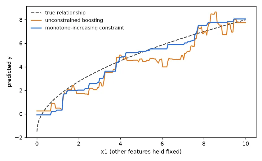
The figure uses synthetic data where the true effect of is , plus noise. The unconstrained model (orange) changes direction dozens of times. The constrained model (blue) is a staircase that only climbs. It’s still a tree model, so it’s piecewise constant, but now its shape matches what we know.
How the library enforces it
The constraint is applied while each tree grows, not as a clean-up step afterwards. The idea, as the XGBoost and LightGBM docs describe it, has two parts.
1. Reject splits that go the wrong way. Say feature has to be increasing, and a candidate split sends to the left child and to the right. Each child has a best leaf value, and (for squared loss, roughly the mean residual in that child). The split is only allowed if . Splits that would make the prediction drop as goes up get thrown out (or the values get clipped).
2. Pass bounds down the tree. This is the part I missed at first: checking one split isn’t enough. A later split deep in the left subtree could create a leaf with a higher value than some leaf in the right subtree. To stop that, after a valid split on the algorithm picks a bound between and (for example their midpoint). Every leaf under the left child is capped at from above, and every leaf under the right child is kept at or above. The final model is a sum of trees, and a sum of monotone functions is monotone, so the whole ensemble respects the constraint.
LightGBM has stricter and looser versions of step 2 (monotone_constraints_method = basic, intermediate, advanced). The looser bounds let the trees fit more detail and still keep the guarantee.
Trying it out
You give the constraints as one number per feature: for increasing, for decreasing, for no constraint. The parameter name depends on the library (monotone_constraints in XGBoost, LightGBM and CatBoost; monotonic_cst in scikit-learn), but the idea is the same. Here’s a small experiment with scikit-learn’s histogram gradient boosting on synthetic data with 300 noisy training rows:
import numpy as np
from sklearn.ensemble import HistGradientBoostingRegressor
from sklearn.metrics import root_mean_squared_error as rmse

rng = np.random.default_rng(0)
def make_data(n):
    x1 = rng.uniform(0, 10, n)            # true effect: increasing
    x2 = rng.uniform(0, 10, n)            # true effect: decreasing
    x3 = rng.normal(0, 1, n)              # no fixed direction
    y = 3 * np.sqrt(x1) - 0.3 * x2 + np.sin(2 * x3) + rng.normal(0, 1.5, n)
    return np.column_stack([x1, x2, x3]), y

X_tr, y_tr = make_data(300)               # small, noisy training set
X_te, y_te = make_data(5000)

params = dict(max_iter=300, learning_rate=0.1, random_state=0)
free = HistGradientBoostingRegressor(**params).fit(X_tr, y_tr)
mono = HistGradientBoostingRegressor(monotonic_cst=[1, -1, 0], **params).fit(X_tr, y_tr)
print(f"unconstrained test RMSE {rmse(y_te, free.predict(X_te)):.3f}")   # 1.781
print(f"monotone      test RMSE {rmse(y_te, mono.predict(X_te)):.3f}")   # 1.666
And a direct check that the guarantee holds:
# Sweep x1 with the other features fixed and count steps that go down
grid = np.linspace(0, 10, 200)
probe = np.column_stack([grid, np.full(200, 5.0), np.zeros(200)])
for name, m in [("unconstrained", free), ("monotone", mono)]:
    steps = np.diff(m.predict(probe))
    print(f"{name:13s} downward steps along x1: {(steps < -1e-9).sum()}")  # 44 vs 0
The constrained model is more accurate on new data and has no reversals. The gain comes from regularization: the constraint rules out a big set of noisy shapes the model could otherwise fit. With lots of clean data the accuracy gain gets smaller, but the guarantee is still there.
When it helps, and when it hurts
Good reasons to constrain a feature:
- Physics, biology or business logic fixes the direction, and you’re confident it holds over the whole input range.
- The training data is small or noisy, so the model needs regularization.
- People (users or regulators) will inspect the model. “A larger value never lowers the score” is easy to explain and easy to test.
- You expect inputs near the edge of the training range, where unconstrained trees are least reliable.
Ways it can go wrong:
- The direction is only true on average. If the real effect goes up and then down (a hump), a monotone constraint forces the model to flatten one side. That’s bias, not regularization.
- Correlated features. If two features carry the same information with opposite signs in the model, constraining one can push the model to use the other in a weird way. Look at related features together.
- Transformed inputs. The constraint applies to the feature as the model sees it. If you feed in instead of , the direction flips. Ratios and differences of features need their own thinking.
- Interactions. The constraint has to hold for every setting of the other features. If the true direction of depends on another feature, no single global constraint is right.
A habit that makes sense to me: compare the constrained and unconstrained models under the same honest validation (grouped folds if the data is grouped). If the constrained one is no worse, prefer it, since it’s the safer model to use.
Key takeaways
- A monotonic constraint forces predictions to move in one direction along a feature, with all the other features held fixed.
- Boosting libraries enforce it during training: they reject wrong-direction splits and pass value bounds down each tree.
- It works as strong regularization based on what you already know: smoother models you can trust more, often with better accuracy on small or noisy data.
- Only constrain directions you’re sure of across the whole range, and remember that transforms and correlated features change what “direction” means.
Resources
- XGBoost documentation, “Monotonic Constraints”: https://xgboost.readthedocs.io/en/stable/tutorials/monotonic.html
- LightGBM documentation, parameters
monotone_constraintsandmonotone_constraints_method: https://lightgbm.readthedocs.io/en/latest/Parameters.html#monotone_constraints - CatBoost documentation, training parameter
monotone_constraints: https://catboost.ai/docs/en/references/training-parameters/common#monotone_constraints - scikit-learn User Guide, “Monotonic Constraints” for histogram gradient boosting: https://scikit-learn.org/stable/modules/ensemble.html#monotonic-constraints
- Maya Gupta et al., “Monotonic Calibrated Interpolated Look-Up Tables”, JMLR 17 (2016), on why monotonicity aids trust and generalization: https://jmlr.org/papers/v17/15-243.html
- Christoph Molnar, Interpretable Machine Learning, chapters on partial dependence and ICE plots: https://christophm.github.io/interpretable-ml-book/
- Jerome H. Friedman, “Greedy function approximation: A gradient boosting machine”, Annals of Statistics 29(5) (2001): https://doi.org/10.1214/aos/1013203451