An MLP language model: embeddings, context windows and honest evaluation

My bigram model only looks at one character, and its made-up names showed it. The obvious fix is more context. But you can’t just make the count table bigger, because the number of rows explodes. Bengio and colleagues had a neat way around this back in 2003. Give every token a small learned vector (an embedding). Glue together the vectors of the last few tokens. Let a neural network turn that into probabilities for the next token. Here I build that model for characters, plus the training habits that came with it.

The dataset: a sliding window of context

First, how do the training examples look now? Pick a context length, block_size = 3. For every position in every name, the input is the three characters before it and the target is the next one. At the start of a name there’s nothing before it, so we pad on the left with the special token . (index 0).

block_size = 3

def build_dataset(words):
    X, Y = [], []
    for w in words:
        context = [0] * block_size
        for ch in w + ".":
            ix = stoi[ch]
            X.append(context)
            Y.append(ix)
            context = context[1:] + [ix]   # slide the window by one
    return torch.tensor(X), torch.tensor(Y)

For emma this gives five examples: ... → e, ..e → m, .em → m, emm → a, mma → .. Over all the names that’s 228,146 examples, each one a row of 3 integers.

The model

The network has three parts.

1. Embedding table C of shape (27, d). Row $i$ is the vector for token $i$. Indexing C[X] turns a (batch, 3) tensor of integers into a (batch, 3, d) tensor of vectors. It’s the same as multiplying one-hot vectors by C, just much cheaper.
2. Hidden layer: flatten the three vectors into one vector of length $3d$, then apply a linear map and a $\tanh$.
3. Output layer: a linear map to 27 logits (raw scores), then softmax inside the cross-entropy loss.

$$h = \tanh\big(\,[e_{t-3}; e_{t-2}; e_{t-1}]\, W_1 + b_1\big), \qquad \text{logits} = h\,W_2 + b_2$$

Here $e_{t-k}$ is the embedding of the token $k$ steps back, $[\,;\,]$ means gluing vectors together, $W_1$ has shape $(3d, H)$ for $H$ hidden units, and $W_2$ has shape $(H, 27)$.

g = torch.Generator().manual_seed(2147483647)
d, H = 2, 100
C  = torch.randn((27, d), generator=g)
W1 = torch.randn((block_size * d, H), generator=g)
b1 = torch.randn(H, generator=g)
W2 = torch.randn((H, 27), generator=g)
b2 = torch.randn(27, generator=g)
parameters = [C, W1, b1, W2, b2]
for p in parameters:
    p.requires_grad = True

def forward(X):
    emb = C[X]                                   # (B, 3, d)
    h = torch.tanh(emb.view(-1, block_size * d) @ W1 + b1)
    return h @ W2 + b2                           # (B, 27) logits

emb.view(-1, 6) flattens the last two dimensions without copying anything. This was new to me. A PyTorch tensor is really a flat block of memory plus a shape and strides, which say how far to jump in memory along each dimension. view only changes that description, so it’s almost free. Gluing emb[:, 0], emb[:, 1] and emb[:, 2] with torch.cat gives the same result, but it uses new memory and hard-codes the context length.

For the loss, use F.cross_entropy(logits, Y) instead of writing softmax and log by hand. Same value, less memory, and it’s numerically safe: it subtracts the biggest logit before taking the exponential, so large logits don’t overflow to inf.

Minibatches

Pushing all 228,146 examples through the model at every step is slow. And you don’t need the exact gradient anyway. Picking 32 random rows per step gives a noisy but good-enough gradient, and you can take many more steps in the same time.

for step in range(15000):
    ix = torch.randint(0, Xtr.shape[0], (32,))
    loss = F.cross_entropy(forward(Xtr[ix]), Ytr[ix])
    for p in parameters:
        p.grad = None
    loss.backward()
    lr = 0.1 if step < 10000 else 0.01        # step decay near the end
    for p in parameters:
        p.data -= lr * p.grad

Finding a learning rate

Then the usual question: what learning rate? Here’s a quick trick. Over 1,000 steps, grow the rate exponentially from $10^{-3}$ to $10^{0}$ and write down the loss at each step. Then plot the loss against the exponent.

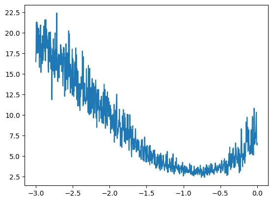
The loss drops fastest and is lowest around $10^{-1}$, then gets unstable as the rate gets close to 1. So 0.1 is a good place to start. Late in training, cutting it by 10x lets the model settle into a lower loss.

Train, dev and test splits

A big model can just memorize its training set. Then a low training loss tells you nothing about how it does on names it has never seen. The fix is to shuffle the words and split them:

• train (80%) to fit the parameters,
• dev or validation (10%) to choose settings like embedding size, hidden size and learning rate,
• test (10%) to report a final number, and only use it rarely.

import random
random.seed(42)
random.shuffle(words)
n1, n2 = int(0.8 * len(words)), int(0.9 * len(words))
Xtr, Ytr = build_dataset(words[:n1])     # 182,625 examples
Xdev, Ydev = build_dataset(words[n1:n2]) # 22,655
Xte, Yte = build_dataset(words[n2:])     # 22,866

How do you read the two losses? If the train loss is clearly lower than the dev loss, the model is overfitting. If they’re about the same but both still high, it’s underfitting: it’s too small, or something else is holding it back.

With 2-dimensional embeddings and 500 hidden units, my train and dev losses stayed close and the test loss was about 2.52. That’s no better than the bigram model (about 2.45). So, underfitting. It took me a moment to see why. The 2-dimensional embedding table was the bottleneck: 3 characters x 2 numbers is very little information for the hidden layer to work with. In the follow-up notebook, 10-dimensional embeddings with 200 hidden units and a better initialization brought the dev and test losses down to about 2.25. That initialization story is in Getting initialization right.

What the embeddings learn

With $d = 2$ you can plot the embedding table directly.

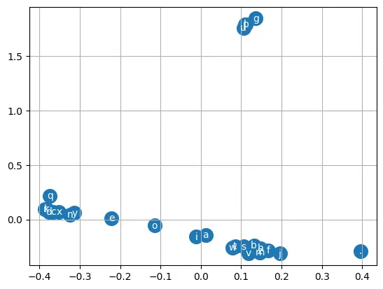
This is my favourite part. Nobody told the network that vowels are similar. They end up close together anyway, because they show up in similar places and can stand in for each other when predicting. The start/end token sits off on its own. And that’s the whole point of embeddings: tokens that behave alike get similar vectors, so what the model learns about one carries over to the others.

Sampling

Generating works like before, except the model now keeps a window of three tokens.

for _ in range(5):
    out, context = [], [0] * block_size
    while True:
        probs = F.softmax(forward(torch.tensor([context])), dim=1)
        ix = torch.multinomial(probs, num_samples=1, generator=g).item()
        context = context[1:] + [ix]
        if ix == 0:
            break
        out.append(itos[ix])
    print("".join(out))

Samples like kay, karin, renly and zayed look a lot more like names than the bigram’s output did.

Key takeaways

• An embedding table gives each token a learned vector. Indexing C[X] is just a fast version of one-hot times matrix.
• Gluing together the embeddings of the last few tokens and feeding them to an MLP lets the context grow without a table that explodes in size.
• Use F.cross_entropy for stability and speed, minibatches for fast steps, and a learning-rate sweep to pick a starting rate.
• Always judge a model on data it hasn’t trained on. Use the dev split for decisions and the test split for the final number.
• Tiny embeddings can be the bottleneck. Going from 2 to 10 dimensions gave the biggest improvement here.

Resources

• Andrej Karpathy, “Building makemore Part 2: MLP”, Neural Networks: Zero to Hero (video): https://www.youtube.com/watch?v=TCH_1BHY58I. The model and training loop here are adapted from this lecture.
• Yoshua Bengio et al., “A Neural Probabilistic Language Model”, JMLR 3 (2003): https://www.jmlr.org/papers/volume3/bengio03a/bengio03a.pdf
• Edward Z. Yang, “PyTorch internals” (strides, storage and views): http://blog.ezyang.com/2019/05/pytorch-internals/
• Andrej Karpathy, makemore (repository): https://github.com/karpathy/makemore