Feature Pyramid Networks: strong features at every scale

One photo can have a 20-pixel bird and a 600-pixel bus in it, and the detector has to find both with the same weights. A CNN backbone gives you sharp, high-resolution maps early on and blurry but “smart” maps at the end. Neither one is good at both jobs. A Feature Pyramid Network (FPN) is a cheap fix: it pushes the smart deep features back into the sharp early maps, so every scale ends up with features that are both detailed and meaningful.

The scale problem, and what people did before

Object sizes in real images can differ by 30 times or more. Before FPN there were three usual answers, and each one had a catch:

1. Image pyramid. Resize the image to several sizes and run the whole network on each one. It works well, but every extra size costs more time and memory.
2. Just the last feature map. Only use the final backbone map (stride 16 or 32), like the first Faster R-CNN did. It’s fast, but a 16-pixel object is smaller than one cell of a stride-32 map, so small objects mostly disappear.
3. Predict from several backbone stages directly, like SSD. This costs nothing extra, because the backbone already computes those maps. The catch is that early maps are high resolution but don’t “understand” much yet. They’ve only been through a few layers, so they react to edges and textures more than to “car” or “dog”.

FPN keeps the low cost of option 3 and fixes its weak spot.

Bottom-up, top-down, and the side connections

The backbone (say a ResNet) is the bottom-up pathway. Its stages give maps $C_2, C_3, C_4, C_5$ with strides 4, 8, 16 and 32 relative to the input. Stride here just means how many input pixels apart two neighbouring cells of the map are. (How to pull these maps out of a backbone is in the backbone note.)

FPN adds a top-down pathway. It starts at the coarsest map and walks back down to the finer ones:

1. A lateral (side) $1\times1$ convolution brings each $C_i$ to the same width, usually 256 channels.
2. The running top-down map is upsampled by 2 (nearest neighbour) so it matches the size of the next finer level.
3. The two are added element by element.
4. A $3\times3$ convolution smooths the sum. The FPN paper adds it to clean up the aliasing (blocky artefacts) that upsampling causes. Its output is the pyramid level $P_i$.

In symbols, with $M_5 = L_5(C_5)$:

$$M_i = L_i(C_i) + \text{Up}_2(M_{i+1}), \qquad P_i = S_i(M_i)$$

where $L_i$ is the lateral $1\times1$ conv, $\text{Up}_2$ is $2\times$ nearest-neighbour upsampling and $S_i$ is the $3\times3$ smoothing conv. The way I think about it: the side path brings where things are (precise edges), and the top-down path brings what they are. Each $P_i$ gets both.

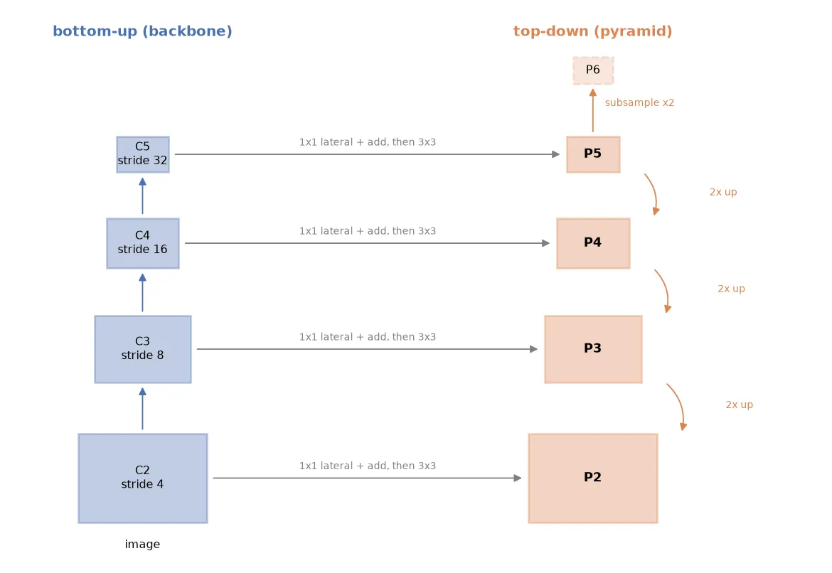
A lot of detectors add one more, even coarser level. Faster R-CNN with FPN makes $P_6$ by subsampling $P_5$ with stride 2, and only uses it to propose very large boxes. RetinaNet does it differently: it makes $P_6$ and $P_7$ with stride-2 $3\times3$ convolutions starting from $C_5$.

A tiny FPN in PyTorch

The module below is really the whole idea. The backbone features are just random tensors with the shapes a ResNet-50 gives for a $512\times512$ input, so the snippet runs without downloading any weights.

import torch, torch.nn as nn, torch.nn.functional as F

class FPN(nn.Module):
    def __init__(self, in_channels=(256, 512, 1024, 2048), out_channels=256):
        super().__init__()
        self.lateral = nn.ModuleList(nn.Conv2d(c, out_channels, 1) for c in in_channels)
        self.smooth = nn.ModuleList(nn.Conv2d(out_channels, out_channels, 3, padding=1)
                                    for _ in in_channels)

    def forward(self, feats):                      # feats = [C2, C3, C4, C5], fine -> coarse
        m = self.lateral[-1](feats[-1])            # start at the top: M5
        outs = [self.smooth[-1](m)]                # P5
        for c, lat, smooth in zip(feats[-2::-1], self.lateral[-2::-1], self.smooth[-2::-1]):
            m = lat(c) + F.interpolate(m, size=c.shape[-2:], mode="nearest")
            outs.insert(0, smooth(m))              # P4, P3, P2
        outs.append(F.max_pool2d(outs[-1], kernel_size=1, stride=2))  # P6: every 2nd cell of P5
        return outs                                # [P2, P3, P4, P5, P6]

H = W = 512
feats = [torch.randn(1, c, H // s, W // s)
         for c, s in zip((256, 512, 1024, 2048), (4, 8, 16, 32))]
with torch.no_grad():
    pyramid = FPN()(feats)
for name, p in zip(["P2", "P3", "P4", "P5", "P6"], pyramid):
    print(name, tuple(p.shape), "stride", H // p.shape[-1])

Output:

P2 (1, 256, 128, 128) stride 4
P3 (1, 256, 64, 64) stride 8
P4 (1, 256, 32, 32) stride 16
P5 (1, 256, 16, 16) stride 32
P6 (1, 256, 8, 8) stride 64

Two small details are worth remembering. First, upsampling to c.shape[-2:] instead of a fixed factor of 2 means the module still works when the input size isn’t a multiple of 32 (odd sizes get rounded differently at each stage). Second, a max-pool with kernel 1 and stride 2 isn’t really pooling. It just keeps every second cell. That’s exactly the “subsample $P_5$” rule from the paper, which confused me the first time I saw it.

Same width everywhere, so the heads can be shared

Every $P_i$ has the same number of channels, and that’s on purpose. Because all the levels look alike, one detection head can run on all of them with the same weights. It’s like an image pyramid, but computed inside the network. The head learns “what an object looks like compared to the cell size”, and picking the level takes care of the actual size. Sharing also means the head gets training examples from every level, which helps with sizes that don’t show up often.

Which level handles which object size

A pyramid only helps if each object gets handled at a sensible level. This choice happens in two places.

Anchors and dense heads. In an RPN or RetinaNet, each level gets anchors of one base size that grows with its stride. The FPN paper uses anchor areas $32^2, 64^2, 128^2, 256^2, 512^2$ on $P_2$ to $P_6$, so the anchor side is 8 times the stride. Small objects end up on fine levels simply because only the small anchors there overlap them well. More on this in the anchors and RPN note.

Region features in two-stage detectors. Once the proposals exist, each region of interest (RoI) of width $w$ and height $h$ is pooled from one level $k$:

$$k = \left\lfloor k_0 + \log_2\!\left(\frac{\sqrt{wh}}{224}\right) \right\rfloor$$

Here 224 is the ImageNet pre-training size and $k_0 = 4$, so a $224\times224$ box reads from $P_4$. Halve the box side and it moves one level finer; double it and it moves one level coarser. The result is clamped to the levels that exist ($P_2$ to $P_5$; $P_6$ is only used for proposals).

import math

def roi_level(w, h, k0=4, canonical=224, k_min=2, k_max=5):
    k = math.floor(k0 + math.log2(math.sqrt(w * h) / canonical + 1e-8))
    return min(max(k, k_min), k_max)

for side in [16, 64, 112, 160, 224, 448, 900]:
    print(f"{side:4d} px box -> P{roi_level(side, side)}")

  16 px box -> P2
  64 px box -> P2
 112 px box -> P3
 160 px box -> P3
 224 px box -> P4
 448 px box -> P5
 900 px box -> P5

So basically, the rule keeps the pooled grid (for example $7\times7$) covering a similar number of cells per object, whatever the object’s size. One thing to keep in mind: if all your objects are small, most RoIs land on $P_2$ and the coarse levels barely do anything. That’s useful to know when picking the input resolution or thinking about dropping levels.

Trade-offs and later versions

• Cost. FPN only adds a few convolutions, but now the heads run on many more cells. $P_2$ alone has 16 times as many cells as $P_4$. On large images, most of the time and memory goes into the finest level.
• Information only flows top-down. Fine levels get meaning from above, but coarse levels never get precise location from below. PANet adds an extra bottom-up path after the FPN to fix that, and BiFPN (EfficientDet) repeats weighted top-down and bottom-up passes.
• Nearest-neighbour upsampling is simple and has no parameters. The $3\times3$ smoothing conv cleans up its blocky output.

Key takeaways

• Early backbone maps are sharp but don’t understand much; late maps understand a lot but are coarse. FPN gives every level both.
• The recipe: $1\times1$ side conv, $2\times$ upsample from the level above, add, then a $3\times3$ smoothing conv.
• All levels have the same number of channels, so one head with shared weights can run on every level.
• Object size decides the level: anchor sizes grow with stride (about 8× the stride), and RoIs use $k = \lfloor 4 + \log_2(\sqrt{wh}/224) \rfloor$.
• The finest level eats most of the compute; coarse levels can sit almost idle if all your objects are small.

Resources

• Lin, Dollár, Girshick, He, Hariharan, Belongie, “Feature Pyramid Networks for Object Detection”, CVPR 2017. arXiv:1612.03144
• Ren, He, Girshick, Sun, “Faster R-CNN: Towards Real-Time Object Detection with Region Proposal Networks”, NeurIPS 2015. arXiv:1506.01497
• Lin, Goyal, Girshick, He, Dollár, “Focal Loss for Dense Object Detection” (RetinaNet, $P_6$/$P_7$ from $C_5$), ICCV 2017. arXiv:1708.02002
• Liu, Qi, Qin, Shi, Jia, “Path Aggregation Network for Instance Segmentation”, CVPR 2018. arXiv:1803.01534
• torchvision.ops.FeaturePyramidNetwork, a ready-made implementation: PyTorch docs
• Related notes: backbone feature extraction, panoptic segmentation (Panoptic FPN builds on this pyramid).